For instrumentation engineers, calibration technicians, and EPC professionals working in oil, gas, chemical, petrochemical, and power sectors, this advanced quiz assesses your real-world expertise in DP transmitter calibration within both workshop and field environments.
Quiz Focus Areas:
HART communicator configuration
Zero and span adjustment
Wet leg and dry leg compensation
Square root extraction
Impulse line effects
Loop diagnostics
Scenarios reflect common calibration challenges in oil, gas, petrochemical, and power plants, including:
Live process isolation
Calibration using deadweight testers
Troubleshooting grounding issues
Calculation-based questions reinforce your understanding of DP-to-flow conversion and loop resistance, enhancing your technical knowledge and problem-solving skills.
Benefits: This quiz helps professionals improve accuracy, reliability, and compliance during DP transmitter calibration ensuring safe, efficient process measurement in critical industrial applications worldwide.
Start The Advanced DP Transmitter Calibration Quiz
Why Plants Use Multiple Transmitters for the Same Measurement
Multiple transmitters for a single process variable are not redundancy for redundancy’s sake they are deliberate engineering choices to control risk, maintain production continuity and meet functional safety obligations. In continuous and semi-continuous process industries (oil & gas, petrochemical, fertilizer, power), a single lost or biased measurement can cause process excursions, spurious trips or prolonged shutdowns.
This article provides practical guidance on why multiple transmitters are used, how different MooN voting architectures behave, the quantitative link to SIL via PFDavg calculations, and field-proven implementation practices and pitfalls all targeted at EPC instrumentation engineers and I&E specialists who must make defensible, auditable design choices.
Key Reasons for Using Multiple Transmitters in Process Industries
Continuity of Operation and High Availability in Process Plants
Objective: minimise unplanned shutdowns and operator interventions.
Mechanism: redundant channels provide immediate failover so control and protection functions continue when one device stops or produces bad data.
Example: in a gas compressor suction control, loss of flow or pressure measurement can force a trip; a 1oo2 or 2oo3 sensing architecture keeps the loop active while maintenance is scheduled.
Metric impact: redundant sensing reduces mean time to failure exposure and increases calculated availability (e.g., % uptime), which can be translated into production-loss dollars in the business case.
Maintenance and Calibration Without Process Shutdown
Objective: perform calibration/repair without halting a process unit.
How it is implemented: use MooN architectures that allow one channel out for calibration while others maintain the safety/control decision. Include hot-swap or exchange kits and procedural steps (isolation, tagging, SIS bypass if required) in the operations manual.
Practical notes: ensure mechanical tappings and manifolds permit individual instrument isolation without impacting measurement fidelity on remaining channels.
Increased Confidence in Measurement for Control and Safety
Objective: detect bias, drift and installation errors early.
Methods: cross-comparison logic, plausibility checks, statistical filtering and trend alarms. Multiple transmitters allow the system to detect a slowly drifting transmitter before it becomes a dangerous failure.
Diagnostic Coverage and Proof Testing for Smart Transmitters
Diagnostic coverage (DC): proportion of failures that diagnostics will detect automatically. Higher DC reduces the portion of dangerous undetected failures, lowering PFDavg.
Proof testing: scheduled manual tests detect failures not covered by diagnostics. Define proof-test intervals (Ttest) based on device reliability and consequence.
Documentation: record proof-test procedures and results in the asset/SIL file to demonstrate lifecycle compliance.
Regulatory and Safety Requirements under IEC 61511
IEC 61511 context: redundancy and voting are common design patterns to achieve target SIL through reduced PFDavg.
Lifecycle view: document allocation of safety requirements, architecture justification and verification evidence in the safety requirements specification (SRS) and the safety validation report.
Refer the below link for the Virtual Redundant Transmitter (VRT) in Honeywell Turbomachinery Control Systems
Voting Logic and MooN Architectures in Safety Instrumented Systems
Understanding M out of N (MooN) Voting Logic
MooN meaning: “M out of N” channels must agree to assert an action. For SIS, clarify whether the logic is voting-to-trip (majority required to trip) or voting-to-run (majority required to continue normal operation) the semantics affect spurious trip behaviour and degraded operation modes.
1oo1 Architecture – Simple but No Redundancy
Pros: simplest, minimal hardware and wiring.
Cons: no redundancy; any dangerous failure directly impacts safety function.
1oo2 Architecture – High Availability with Limited Fault Tolerance
Use: where online maintenance and minimal interruptions are prioritized.
Behaviour: system continues with a single healthy channel; but a single faulty channel can increase nuisance trips if voting logic treats inconsistent data as trip condition. Best used with robust plausibility and alarm suppression during transient conditions.
2oo3 Architecture – Preferred Design for High Integrity SIS Loops
Use: high-consequence SIS loops where both availability and low spurious-trip risk are needed.
Behaviour: tolerates a single device failure without loss of protective function; reduces spurious trips by requiring concurrence. Supports graceful degradation.
1oo3 Architecture – Special Cases in Availability Driven Systems
1oo3 increases availability but can be sensitive to majority voting semantics. Evaluate case-by-case.
Impact of Voting Architecture on Spurious Trips and System Availability
Availability vs safety: 1oo2 favours availability; 2oo3 favours safety and robustness to spurious trips.
Complexity: 2oo3 requires more hardware and more extensive CCA because of increased CCF exposure paths.
Operational mode: define explicit degraded-mode SOPs (e.g., alarm when architecture falls to 1oo2).
Safety Integrity Level (SIL) and Reliability Concepts
Understanding SIL Requirements in IEC 61511
PFDavg: average probability that the safety function will fail on demand over the mission/proof-test interval.
SIL mapping: IEC 61511 uses PFDavg bands to assign SIL levels (e.g., SIL 1 to SIL 4 ranges). Achieving SIL is about demonstrating PFD via credible data, diagnostics and architecture.
Worked Example of PFD Calculation for Redundant Transmitters
Assumptions Used for Reliability Calculation
Single transmitter PFDavg (P) = 1 × 10⁻² (0.01).
Independence is assumed between channels (no Common Cause Failure) for the baseline comparison.
Diagnostic functions and proof tests are assumed to be included within the value P.
Reliability Formulas for 1oo1, 1oo2 and 2oo3 Architectures
For redundant architectures, the simplified reliability relationships are:
PFD₁oo₁ = P
PFD₁oo₂ ≈ P² (Both transmitters must fail simultaneously to impair the safety function.)
PFD₂oo₃ ≈ 3 × P² (The combinational factor C(3,2) = 3, meaning any two transmitters out of three must fail.)
Numeric PFD Calculation Example
1oo1 Architecture
PFD₁oo₁ = 1 × 10⁻²
PFD₁oo₁ = 0.0100
1oo2 Architecture
PFD₁oo₂ ≈ (1 × 10⁻²)²
PFD₁oo₂ ≈ 1 × 10⁻⁴
PFD₁oo₂ ≈ 0.0001
2oo3 Architecture
PFD₂oo₃ ≈ 3 × (1 × 10⁻²)²
PFD₂oo₃ ≈ 3 × 1 × 10⁻⁴
PFD₂oo₃ ≈ 3 × 10⁻⁴
PFD₂oo₃ ≈ 0.0003
Interpretation of Results for Different Architectures
A single transmitter with P = 1 × 10⁻² roughly corresponds to SIL 1 capability, depending on the proof-test interval and system design.
A 1oo2 architecture significantly improves reliability because both transmitters must fail simultaneously before the safety function fails. This gives approximately 100× improvement compared with a single transmitter.
A 2oo3 architecture may show a slightly higher theoretical PFD in simplified calculations compared with ideal 1oo2, but it provides important operational advantages such as:
Lower spurious trip probability
Higher fault tolerance
Ability to tolerate one faulty transmitter while maintaining operation
Technology diversity (e.g., radar level transmitter with differential pressure transmitter)
Physical separation of transmitters
Independent impulse lines
Separate power supplies
Separate signal cables and I/O modules
Staggered proof-test intervals
During SIL verification, a Common Cause Analysis (CCA) is performed to justify the selected β-factor and confirm that the redundant architecture genuinely reduces the overall risk.
Implementation Best Practices for Redundant Transmitter Systems
Key Design Principles for EPC Instrumentation Engineers
Technology diversity: radar, DP, ultrasonic where appropriate to reduce shared failure modes.
Physical separation: stagger tappings and manifold locations; avoid common supports that can introduce mechanical CCF.
Independent power and grounding: separate UPS/PSUs and isolated earthing to prevent electrical single-point failures.
Independent signal routing: separate conduits and junction boxes; different cable trays preferred.
Robust diagnostics: require HART/fieldbus diagnostics and ensure diagnostic flags pass to SIS.
Staggered proof tests: avoid simultaneous proof-testing of redundant channels to prevent temporary loss of redundancy.
Vendor Data Requirements for SIL Verification
Request manufacturer λD, DC, MTTR and field failure data; require factory test certificates and detailed diagnostics descriptions. Include acceptance tests for redundancy features.
Practical Case Study – Redundant Flow Measurement for Furnace Protection
Process Scenario and Safety Requirement
Scenario: high-pressure steam header low-flow detection required SIL 2 to prevent furnace damage. Consequence: potential tube overheating and production loss.
Selection of 2oo3 Architecture with Technology Diversity
Chosen architecture: 2oo3 using two vortex flowmeters and one ultrasonic clamp-on (diverse tech). Justification:
Vortex meters provide primary reliable measurement; ultrasonic adds independence and is non-intrusive.
Diversity reduces β and addresses different failure modes (mechanical clogging v. electronics).
Reliability Estimation and Beta Factor Consideration
Per-device P = 1×10^-2, β conservatively estimated 0.03 due to diversity. Approximate 2oo3 combinatorial corrected PFD ~ 4×10^-4 (rounded) after including β and shorter proof-test (T=6 months) and DC improvements.
Maintenance and Diagnostic Monitoring Strategy
Quarterly diagnostic trend review, annual SIS trip proof-test, and immediate exchange of any trending device. Keep hot spare and calibration exchange kit.
Redundant transmitters are a deliberate tool for balancing availability, safety and operational cost.
Use MooN voting, realistic β and DC values, vendor data, and formal SIL verification to justify designs.
Immediate next steps for I&E teams: run a Common Cause Analysis, update loop drawings to show physical independence, and perform SIL verification with documented assumptions.
Implement disciplined proof-test and diagnostics governance to maintain the claimed PFD performance throughout the lifecycle.
FAQ on Redundant Transmitters, CCF, Diagnostics and Proof Testing
What are redundant transmitters in process instrumentation?
Redundant transmitters are several sensors that measure the same process variable to make sure it works better and is safer. They allow systems to continue operating even if one transmitter fails, which is common in SIS and critical control loops.
What is MooN voting logic in transmitter redundancy?
MooN (M-out-of-N) voting logic determines how many transmitters must agree before a control action occurs. For example, 2oo3 voting requires two out of three transmitters to confirm the condition, improving fault tolerance.
What is Common Cause Failure (CCF) in redundant transmitter systems?
Common Cause Failure happens when a shared cause causes more than one redundant transmitter to fail.
Common causes are problems with the shared power supply, clogged impulse lines, or environmental factors like vibration or temperature..
Why are diagnostics important in smart transmitters?
Smart transmitters have built-in diagnostics that can find problems like sensor drift, electronics failure, or mistakes in the configuration. These diagnostics improve safety integrity and help maintenance teams identify problems before process shutdown occurs.
What is proof testing in safety instrumentation systems?
Scheduled proof testing checks that safety devices work correctly.
It helps find hidden problems and keep the protection system’s Safety Integrity Level (SIL) where it needs to be.
Refer the below for the Intrinsic Safety Protection Systems: Understanding Ex ia, Ex ib, and Ex ic
Ethernet APL is the process industry adaptation of single pair Ethernet that carries data and in many cases device power on a single balanced pair while supporting intrinsic safety in classified zones. For EPC teams this means simpler wiring fewer marshalling points and native Ethernet connectivity at the device edge. This guide focuses on practical fundamentals design checks installation rules wiring best practice commissioning step lists migration patterns and troubleshooting notes you can apply on greenfield and brownfield projects.
What is Ethernet-APL and 10BASE-T1L?
Ethernet APL is a physical layer solution aimed at process industry needs rather than office LAN environments. It is built on a long reach single pair PHY often referenced as 10BASE T1L that supports 10 Mbit s throughput over a single balanced conductor pair. Key basic concepts expanded
Ethernet APL uses one balanced conductor pair per segment instead of two pairs or four pairs found in classic Ethernet. The single pair carries the PHY signal and in many configurations also supplies low voltage power to the device.
Data Rate, Long Reach and Suitability for Process Telemetry
The physical rate is 10 Mbit s which is sufficient for process telemetry diagnostics and asset management while enabling lower complexity cabling and improved reach relative to copper multipair Ethernet.
Two-Wire Power and APL Port Profiles
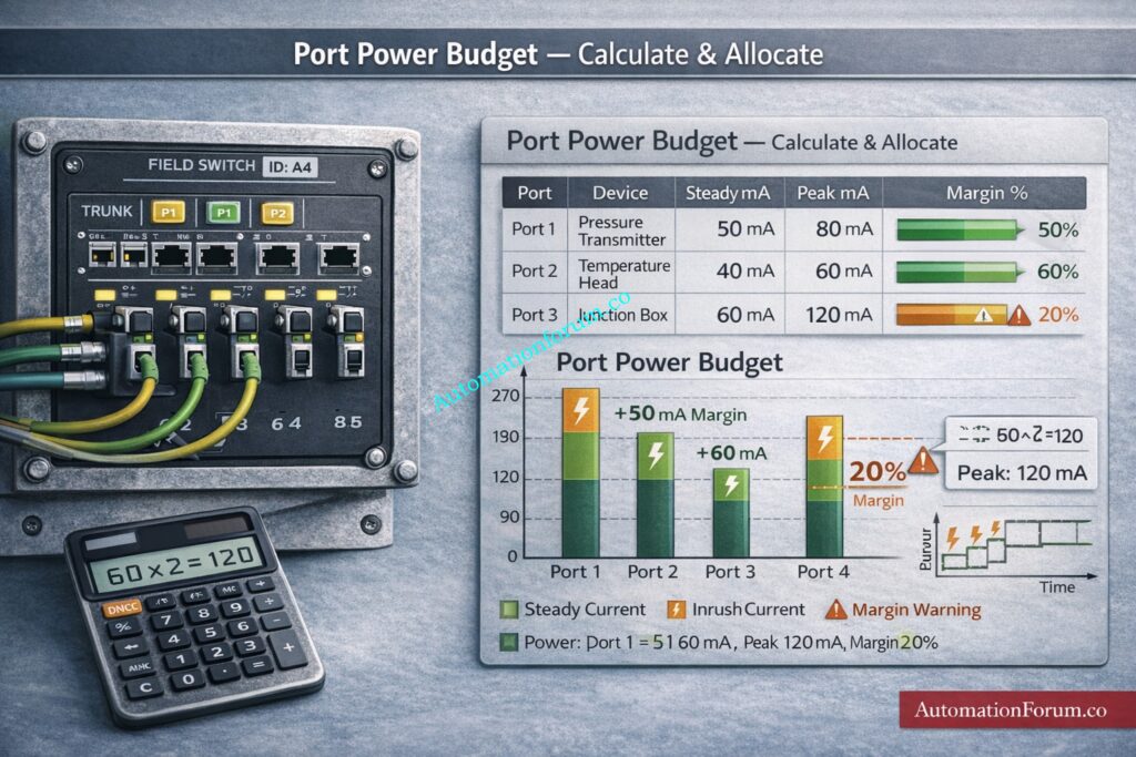
APL defines port power classes and profiles so a field switch port can supply a defined amount of power to attached devices. Designers must allocate port budgets and ensure device draws fall within declared limits.
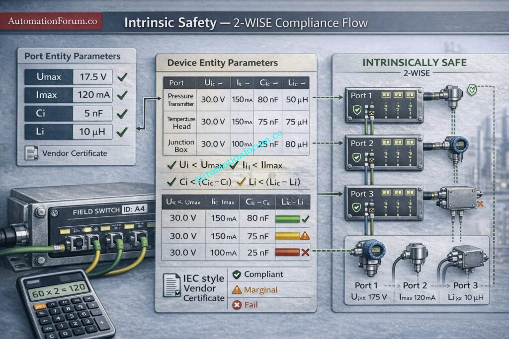
Intrinsic Safety and the 2-WISE Concept
APL supports an intrinsic safety model where device and port entity parameters are declared and checked so the energy available in a circuit remains below ignition thresholds in a classified area. This is commonly referenced as the two wire IS concept or 2 WISE.
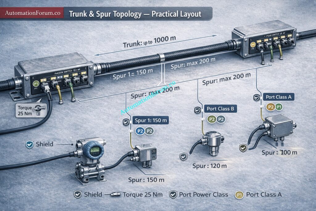
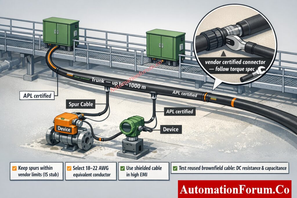
APL deployments commonly use trunk and spur topology. Trunks run between field switch locations while spurs branch to devices. The topology is familiar to fieldbus engineers and simplifies staged migration. Vendors provide port profile data sheets entity parameter tables and zone certificates. Require these documents in procurement to avoid integration surprises.
Protocol Layer Independence and Application Use Cases
APL is a physical layer only. Any standard Ethernet based application protocol can run above it subject to device firmware support. Common use cases are device telemetry remote diagnostics and asset management.
Physical Layer and Cable Topology – Practical Engineering Rules
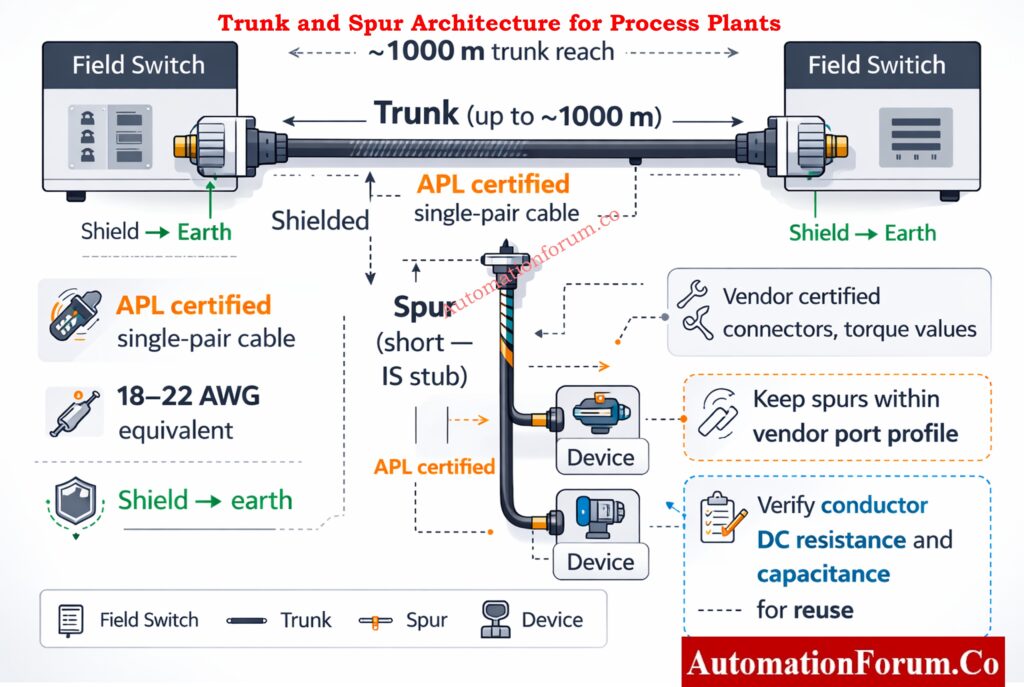
Trunk and Spur Architecture for Process Plants
Trunk and spur remains the practical topology for most plant installations. Below is a compact ASCII diagram showing the concept using characters that do not include hyphen
Maximum Trunk Reach and Environmental Planning
Plan trunks for long reach capacity. Typical design targets use trunks up to around one thousand meters depending on cable category and ambient conditions. Use conservative design values based on cable data and site temperature.
Spur Length Limits and Intrinsic Safety Constraints
Spurs are shorter and in many IS schemes are treated as stubs with tighter limits. Keep spurs within recommended lengths from the port profile or vendor document to avoid violating entity parameter assumptions.
Cable Selection, Conductor Sizing and Voltage Drop Considerations
Specify APL certified single pair cable types and conductor sizes sized for mechanical durability and power drop. Conductor equivalents in the 18 to 22 AWG family are common but verify for your run lengths and ambient conditions.
Shielding, Jacket Selection and EMI Protection
Use shielded variants for high EMI environments and specify jacket chemistry and temperature rating for the process. Shield drain wiring must terminate to earth at the enclosure point chosen by the site earthing plan.
Use vendor certified APL rated connectors and follow termination torque values exactly. Use strain relief and ingress seals suitable for the zone and environmental rating.
Reusing Existing Fieldbus Cable in Brownfield Projects
Reuse is possible but only after verification of conductor gauge insulation capacitance and DC resistance against the port profile. Test each run and document acceptance.
APL enables power over the same pair in a controlled manner via port power classes. For EPC design follow these rules
Port Power Budget Calculation Method
For every field switch maintain a power budget sheet that lists the available trunk power per switch and allocates per port. Include steady state draw and peak draw and keep a design margin typically twenty percent for growth and inrush.
Device Selection Criteria for Spur Powering
Small transmitters and smart sensors can be powered by APL spurs. Heavy devices such as motorized actuators and large valve positioners normally require local mains or local DC and must be excluded from spur powering unless explicitly supported by the port class.
Managing Inrush Current and Startup Sequencing
Account for device inrush currents at boot. Implement sequential connection of spurs during commissioning so multiple devices do not draw peak current simultaneously and trigger power limiting.
Where multiple devices cluster use APL powered junction boxes or small distribution enclosures that report into the port profile while providing local terminations.
Equipotential Bonding and Shield Termination Strategy
Establish equipotential bonding for field enclosures and terminate shields as defined by the site earthing plan. Don’t use floating shields that let EMI in.
Routing Separation from Power Cables
Don’t let APL trunks touch power lines. To cut down on inductive and capacitive coupling, use different trays or pathways.
Surge Protection Device Placement for APL Networks
Put surge protecting devices that work with APL at marshalling and switch sites, but make sure that the SPD characteristics stay within the entity parameter limitations.
Enclosure grounding and SPD placement
Ground shields and protective earth at designated enclosure points. Place SPDs at the boundary where they protect but do not interfere with the intrinsic safety mapping.
Zone Planning and Field Switch Installation Guidelines
Locate field switches and marshalling according to zone classification and use devices certified for the appropriate zone.
Migration Strategies for Greenfield and Brownfield Projects
Practical migration paths for EPC projects
Greenfield APL-Native Design Approach: Design APL from the outset place field switches near device clusters reduce marshalling and simplify future expansions.
Brownfield Migration from FOUNDATION Fieldbus or 4–20 mA HART: Deploy APL in parallel with legacy 4 20 mA HART or other fieldbus systems. Use gateways for protocol translation while replacing loops during planned outages.
Hybrid Architectures with Gateways and Legacy Coexistence: Place managed APL field switches at the edge and use gateway devices to the DCS or asset management systems. Keep legacy loops until replacement is scheduled.
Planning and Scheduling for Phased Migration: To minimize downtime and keep spare parts and resources, plan the order in which devices will be replaced based on how important they are to safety and how they are physically grouped.
Diagnostics, Maintenance and Troubleshooting Guide
Common Failure Modes in Ethernet-APL Networks
Cable open or break: Link down symptom: no device discovery Action: isolate the section, measure continuity, and replace the cable if necessary.
Power Budget Errors and Brownout Conditions: Symptom: the device goes dark or restarts Action check port reports lower the load on the attached device or raise the supply capacity.
EMI and Grounding Related Packet Errors: Symptom Intermittent packet errors and CRC Action verify shield bonding and cable routing separation from power runs.
Diagnostic Logs to Capture and Archive
LLDP neighbor tables and link state snapshots
Port power consumption logs and switch reported events
Packet capture of device boot and application traffic during failure.
Case Study 1 – Brownfield Retrofit Replacing FOUNDATION Fieldbus
Problem: congested mechanical conduits and limited pull space.
Approach: reuse Type-A FF cable where permitted, install intrinsically safe APL power-limiting switches in marshalling, and deploy protocol gateways for coexistence during phased migration.
Outcome: minimized hook-up changes, maintained IS boundaries, and staged device replacement to control spend.
Case Study 2 – Greenfield Chemical Plant Using Ethernet-APL
Problem: mixed device classes and long distances.
Approach: define primary trunks in safe corridors with APL switches in marshalling cabinets; calculate worst-case power budgets for simultaneous startup; select suppliers with IEC TS 63444 port profiles and 2-WISE certificates.
Result: easier wiring, better diagnostics, and centralized power control.
Frequently Asked Questions (FAQ) – Ethernet-APL for EPC Engineers
What is the difference between PROFINET and Ethernet APL?
PROFINET is an industrial communication protocol used for controller and device communication in automation systems. Ethernet APL is a physical layer technology that enables Ethernet communication directly to field instruments over a two wire cable. PROFINET and other Ethernet protocols can run over Ethernet APL.
What is APL in network?
APL stands for Advanced Physical Layer. It is a networking technology designed for process industries that allows Ethernet communication and power transmission over a single two wire cable while supporting long distances and hazardous area installations.
How fast is Ethernet APL?
Ethernet APL has a data throughput of 10 Mbps. This speed is best for automating industrial processes since it has enough capacity for device communication, diagnostics, and asset management while still being able to reach long cables.
What is the difference between Ethernet APL and SPE?
Single Pair Ethernet (SPE) is a general Ethernet technology that transmits data over a single pair of wires. Ethernet APL is a specialized implementation of SPE designed for process plants, including long cable reach, power delivery, and intrinsic safety support.
What is the full form of Ethernet APL?
Ethernet APL stands for Ethernet Advanced Physical Layer. It is a physical layer technology that enables Ethernet connectivity to field instruments using a two wire cable infrastructure.
Is Ethernet APL intrinsically safe?
Yes. Ethernet APL uses a two-wire intrinsic safety paradigm to ensure inherently safe operation. This lets Ethernet communication happen in dangerous regions like Zone 1 and Zone 2 in process plants.
What is an APL device?
An APL device is any field instrument designed to communicate using Ethernet APL. Ethernet APL is an APL device. Pressure transmitters, temperature transmitters, flow meters, and field switches that can talk to each other over a two-wire cable are all examples.
Control valve body material selection is a highest-impact decision in global EPC projects across oil & gas, petrochemical, chemical, power, and process industries. Wrong choices result in early field failures, unplanned shutdowns, safety incidents, and dramatically increased lifecycle cost. This control valve material selection guide is written by an instrumentation and materials engineer with EPC field experience to help engineers specify practical, standards-compliant choices during FEED and detailed engineering.
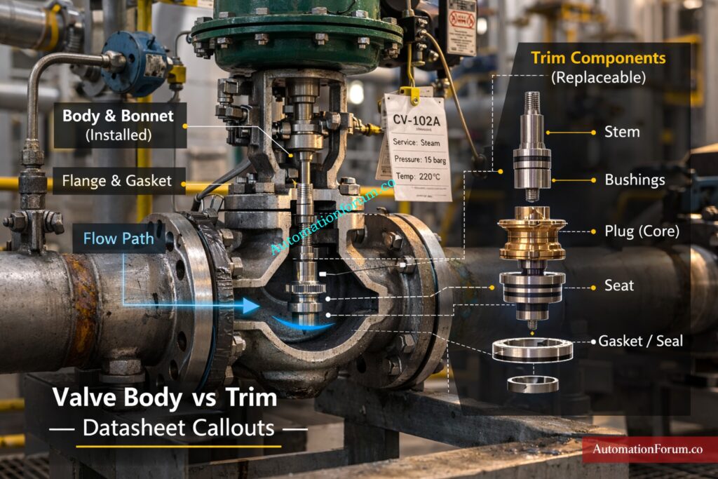
Valve Body Vs Trim Critical Distinction For Datasheets
The valve body material forms the pressure-retaining pressure boundary and provides structural strength, flange/bolt interface, and gross corrosion resistance of the assembly. Trim material (plug, seat, stem, bushings) is the wetted internal working surface that determines erosion, leakage, and sealing performance. Do not conflate the two: stainless trim in a carbon body does not guarantee sour-service compliance or eliminate SSC risk in the body or HAZ. Specify body and trim explicitly in datasheets.
Epc Material Selection Workflow Feed To Detailed Engineering
Process Definition at Feed Stage
Capture maximum pressure, MAWP, operating and design temperatures, expected transients, two-phase conditions, solids content, and full compositional analysis including chlorides, CO₂, and H₂S ppm. Document velocity, particle size, solids concentration, and sand/scale risk. Additionally, confirm design life (typically 20-25 years), corrosion allowance philosophy, shutdown philosophy, and whether the valve is classified as critical, SIL-related, or part of emergency isolation. Early alignment with piping material class and piping line specification is essential to avoid later material conflicts.
Preliminary Material Screening and Cost Categorization
Use corrosion indices, temperature thresholds, and cost buckets (CS, low-alloy, duplex, super duplex, nickel alloys) to produce a short list of body alloys.
Early on, mark seawater, chloride-bearing, and sour-service streams for alloys that won’t corrode.
To avoid underspecification, do a preliminary comparison of the mechanical strength and the required pressure class according to ASME standards.
Risk Assessment Hazop Corrosion Review and Specialist Input
Run HAZOP corrosion nodes and consult corrosion/materials engineers for SCC, SSC, hydrogen embrittlement and cavitation risk mitigation. Look into the history of failures in similar initiatives and use what you learnt from your clients.
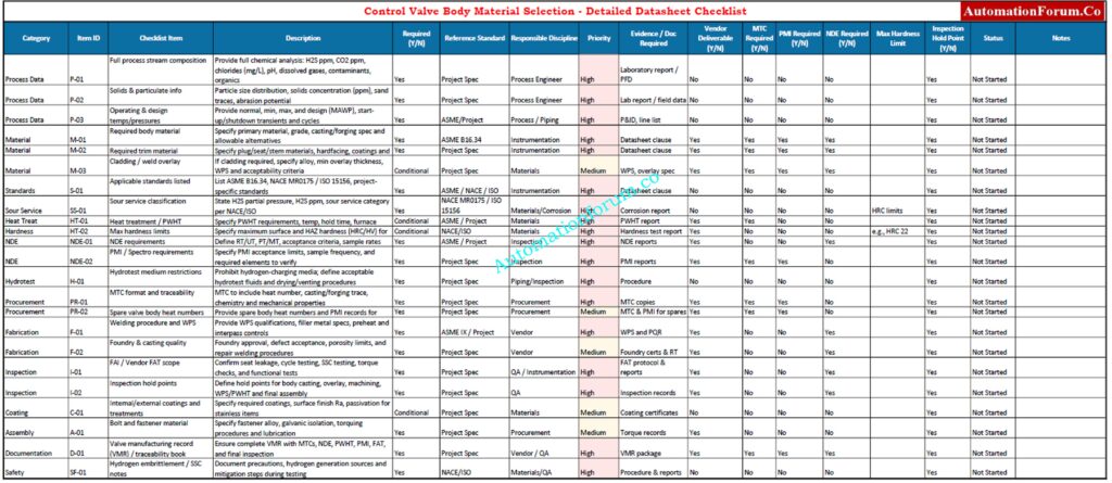
Datasheet Preparation Mandatory Material And Inspection Clauses
List the body and trim materials that the state requires, the alternatives that are allowed, the NACE/ISO sour-service qualification demands, the cladding requirements, the hydrotest medium, and the ways to prevent erosion and cavitation.
Set the highest hardness limits, the coating requirements, and the locations at which inspections must stop.
Vendor Evaluation FAI And Final Engineering Sign Off
For traceability, you need vendor MTC, PMI acceptance criteria, NDE records, cladding/weld overlay procedures, and sample heat numbers.
Check the quality of the casting, the approvals from the foundry, and the steps for repair welding.
Finalize the WPS, PWHT, bolt metallurgy, and acceptance criteria. Make sure that the vendor’s FAI includes seat leakage, cycle testing, and SSC testing as necessary.
Make sure that all paperwork is put together in the valve manufacturing log book for project turnover.
Pressure and temperature: set the limits for stresses and the grade of material to use. High temperatures lower the permitted stress and may require low-alloy chrome-moly (WC6/WC9) instead of plain CS.
Corrosivity: the complete process chemistry (pH, chlorides, oxidants) determines whether to use austenitic, duplex, or nickel alloys.
Velocity and solids: erosion and erosion-corrosion risk favor harder trims, erosion liners, and abrasion-resistant alloys.
Cavitation and flashing: severe erosion risk-use anti-cavitation trims, staged pressure reduction, and consider body materials with erosion resistance.
Slurries and solids: consider lined bodies or hardened inserts and material toughness for impact.
Sour service: H2S presence requires compliance with NACE MR0175 and ISO 15156 rules for hardness, metallurgy, and testing.
Corrosion Mechanisms And Material Selection Implications
Uniform corrosion: predictable; mitigate with corrosion allowance or cladding.
Pitting: a localized assault that happens in situations with chloride; duplex and super duplex resist pitting better than 304/316.
Crevice corrosion: stay away from crevices, use materials that are resistant to crevices, and keep an eye on the materials and surface finish of gaskets.
Stress corrosion cracking (SCC): tensile stress plus the environment; control leftover stresses and choose alloys that won’t crack under stress.
Sulfide stress cracking (SSC) and hydrogen embrittlement are very important for streams that carry H2S. To keep hardness under NACE/ISO limits, you should utilize only approved materials.
Erosion-corrosion: damage from both mechanical and chemical sources; you can reduce it by using hardfacing or bodies and trims that are more resistant to erosion.
High temperature: oxidation, carburization, and lower yield strength need alloys and heat treatment to keep strength and resistance to creep.
Cryogenic: To avoid brittle fracture, utilize austenitic stainless steel, nickel alloys, or cryogenic-rated carbon steels that have been tested for toughness and are compatible with welding consumables.
Seawater: warm seawater causes pitting and crevice corrosion. 304/316 are often inadequate; select duplex, super duplex, or nickel-copper alloys (Monel) for long-term seawater exposure.
Use cathodic protection and coatings only as supplementary measures – choose body alloy for primary compatibility.
Valve Body Material For Sour Service Nace Mr0175 And Iso 15156
For valve body material for sour service ensure selection, hardness limits, testing, and metallurgical controls meet NACE MR0175 and ISO 15156.
Verify vendor SSC test reports, hardness measurements, and MTC traceability. If there is a high risk of H2S or SSC, utilize CRAs instead of just heat treatment.
Do not let different metals touch each other when they are wet or in a chloride atmosphere. Choose materials with similar electrochemical potentials or electrically isolate interfaces. Specify fastener metallurgy consistent with body materials to prevent accelerated corrosion.
Cladding Vs Solid Alloy Bodies Selection Guidelines
Cladding (weld overlay) can provide corrosion resistance inside a lower-cost base metal body when mechanical loads are moderate.
Limitations: cladding delamination, porosity, HAZ susceptibility, and potential inability to meet sour-service SSC requirements if HAZ affects base metal. For severe sour or high-mechanical loads prefer solid alloy bodies.
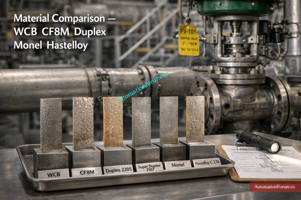
Detailed Material Comparison For Control Valve Bodies
Material
Typical application
Temperature range
Corrosion resistance level
Cost level
Limitations
EPC design / procurement notes
Carbon Steel (WCB)
General service, non-corrosive process lines, utility isolation valves
Cryogenic (with appropriate grade & testing) up to ~425°C (grade dependent)
Low – requires corrosion allowance or protective coating in corrosive services
Low
Poor resistance to chlorides, seawater and sour environments; not suitable for H2S unless fully qualified
Use where economy is priority and process chemistry is benign. Specify MTC, PMI for forgings, and consider internal cladding if moderate corrosion expected.
Low Alloy Steel (WC6 / WC9)
High-temperature steam applications, hydrocarbon services at elevated temperature
Up to ~540°C (depending on grade and thickness)
Moderate better high-temperature strength than plain CS but limited chemical resistance
Moderate
Limited chloride and H2S resistance; susceptible to scaling/oxidation at high T
Select for elevated-temperature service where creep strength is needed. Require PWHT and strict heat-treatment records (MTC + PWHT report).
Stainless Steel 304 / 316 / 316L
Clean water systems, mild chemicals, general corrosion-resistant applications
Cryogenic to ~400°C (316 often preferred at higher T and chloride tolerance)
Moderate – 316/316L > 304 for chlorides; susceptible to localized attack in aggressive chloride environments
Moderate
Vulnerable to pitting/crevice corrosion in warm chloride environments; SSC risk in sour service
Use when moderate corrosion resistance and weldability required. For chloride/seawater service, evaluate duplex or higher alloys. Specify hardness limits and SSC qualification if H2S present.
Duplex Stainless Steel (2205)
Seawater systems, chloride-bearing streams, many oil & gas wetted services
Approx. -50°C to ~300°C (good low T toughness and higher strength)
High – excellent pitting and crevice resistance vs 304/316
High
Requires controlled welding practices and experienced fabrication; limited availability for some sizes
Good balance of strength and corrosion resistance for offshore and chloride environments. Specify PWHT avoidance, qualified WPS, PMI and heat traceability.
Super Duplex (2507)
Aggressive seawater, high chloride CO₂/Cl⁻ environments, high integrity oil & gas applications
Similar to duplex but often with slightly narrower service limits due to fabrication constraints
Very high – superior pitting/crevice and chloride resistance
Very high
More difficult to fabricate/weld; longer lead times; requires experienced suppliers
Use where highest chloride/pitting resistance is needed. Ensure supplier capability for forging/casting and fully documented NDE and MTC.
Alloy 20
Service with acid chlorides and certain sulfuric acid applications; specialty chemical lines
Application dependent (moderate to elevated temperatures per alloy datasheet)
High for specific acidic environments (selected chemistries)
High
Not a universal solution – best for particular acidic chemistries
Specify based on detailed process chemistry. Require vendor corrosion data and MTC confirming composition.
Monel (Alloy 400)
Seawater systems, some acidic environments and mixed media where cu-nickel is desirable
Wide range; consult alloy data for exact limits
High resistance to seawater and many acids
Very high
Costly; magnetic and fabrication considerations
Consider where seawater corrosion plus occasional acid exposure exist. Specify PMI and fabrication experience.
Hastelloy (C-276 / C-22)
Highly corrosive chemistries, oxidizing and reducing acid mixtures, aggressive process chemistries
Broad service ranges per alloy – selected for severe chemical resistance
Excellent – one of the best for mixed acid/oxidizing environments
Extremely high
Very expensive; long lead times; special fabrication/welding practices
Use only when process chemistry justifies cost. Require supplier corrosion test data, full MTC, and tight welding controls.
If you want, I can convert this table into a printable PDF or add columns for material standards (ASTM/EN), typical trim pairings, and maximum allowable hardness for sour service.
Case 1 – Offshore Cooling Water Control Valve Seawater Service
Scenario: a warm seawater cooling line on an offshore platform that runs all the time at 35–40°C and stops working for maintenance every so often.
Analysis:The first FEED step called for 316 stainless steel because the chloride concentration was low. But a thorough corrosion review found that there was a high danger of crevice corrosion at the gasket faces, bolting interfaces, and trim-body clearances. Warm, oxygenated seawater significantly increases pitting potential. Historical data from similar offshore assets showed perforation within 18-24 months for 316 bodies in stagnant sections. There was also a potential of galvanic interaction between the stainless steel body and the carbon steel piping.
Solution: The answer is a Duplex 2205 body and trim with proper welding methods, stringent heat input control, and 100% PMI. It was required to have flange isolation kits and cathodic protection integration.
Rationale: Duplex has a better pitting resistance equivalent number (PREN) and almost twice the yield strength of 316, which lets you use thinner wall sections without losing mechanical strength. Even if the initial cost of buying was higher, calculating the cost of the whole life cycle revealed that big savings could be made by not having to replace things in the middle of their lives or send somebody to work on them from abroad.
Scenario: In a power generation plant, superheated steam is controlled at about 450°C and 45 bar. It was assumed that the load would cycle often.
Analysis: Austenitic stainless steel was first thought of because it doesn’t rust. Mechanical design verification, on the other hand, demonstrated that the stress limit went down at high temperatures and that there was a possibility of long-term creep deformation. Thermal cycling also raised worries about tiredness.
Solution: A WC6 low-alloy chrome-moly steel body with PWHT, creep-strength testing, and hardfaced trim to protect against corrosion.
Rationale: Chrome-moly steel has better creep strength and structural stability at high temperatures for a long time. Proper heat treatment keeps metals stable and stops them from breaking down too soon. The material choice met high-temperature service criteria and made sure that the dimensions stayed stable over time, even when they were used in cycles.
Scenario: An injection control valve that handles hydrocarbons with H₂S and CO₂ and has two-phase flow and sand traces from time to time.
Analysis: There was a high danger of sulfide stress cracking, the possibility of hydrogen embrittlement, and erosion from solids that got stuck in the material. Carbon steel with a corrosion allowance was turned down because it was likely to suffer from SSC. It was necessary to manage hardness and follow metallurgical standards.
Solution: Super duplex or high-nickel alloy, depending on the partial pressure of H₂S. It must meet NACE MR0175’s SSC qualification, hardness verification, and full material traceability.
Rationale: Alloys that don’t rust lower the risk of SSC while keeping their mechanical strength. Choosing the right materials at the design stage kept future risks to integrity from happening and made sure that the sour-service project parameters were met.
It makes sure that process data, material needs, standards compliance, inspection criteria, and vendor documentation are all properly recorded to avoid corrosion failures, sour-service non-compliance, and holes in traceability.
Mill Test Certificates (MTC) show how heat numbers are linked to chemical and mechanical qualities.
PMI/spectro reports on castings and forgings.
NDE records (radiography, UT, PT/MT) with acceptance criteria.
Hardness testing reports on body surfaces and HAZ for sour-service items.
Welding and PWHT records linked to part heat numbers.
Lifecycle Cost Reliability and Maintenance Strategy
Prioritize reliability where control valve body material selection impacts safety, production, or shutdown risk. Upfront alloy cost is frequently small compared to unplanned shutdown expense and repeated maintenance.
Adopt conservative materials for chloride-bearing or sour environments: duplex stainless steel control valve bodies or higher alloys typically reduce total cost of ownership.
Embed material checkpoints in FEED datasheets, vendor queries, FAT, and site commissioning to ensure compliance with standards, testing, and traceability.
Common valve body materials include Carbon Steel WCB, Stainless Steel CF8 and CF8M, Duplex Stainless Steel, Low Alloy Steel WC6 WC9, Cast Iron, Bronze, Monel, Alloy 20, and Hastelloy. Material selection depends on pressure, temperature, corrosion level, and process fluid composition.
What is CF8M Body Material?
CF8M is a cast austenitic stainless steel that is similar to AISI 316 stainless steel but has molybdenum added to make it more resistant to corrosion.
It is frequently utilized in the oil and gas and chemical industries because it is more resistant to chlorides and chemicals than CF8.
What is WCB Material For Valves?
WCB is cast carbon steel that meets the standards of ASTM A216 Grade WCB. It is often used for valve bodies in normal duty applications.
It has good mechanical strength for moderate pressure and temperature, but it doesn’t resist corrosion very well.
What are the Criteria For Control Valve Selection?
The flow rate, pressure drop, kind of fluid, temperature, risk of cavitation, noise level, and level of control accuracy all affect how to choose a control valve.
Material compatibility, pressure rating, actuator type, and safety standards are also very important.
How to Calculate Control Valve Size?
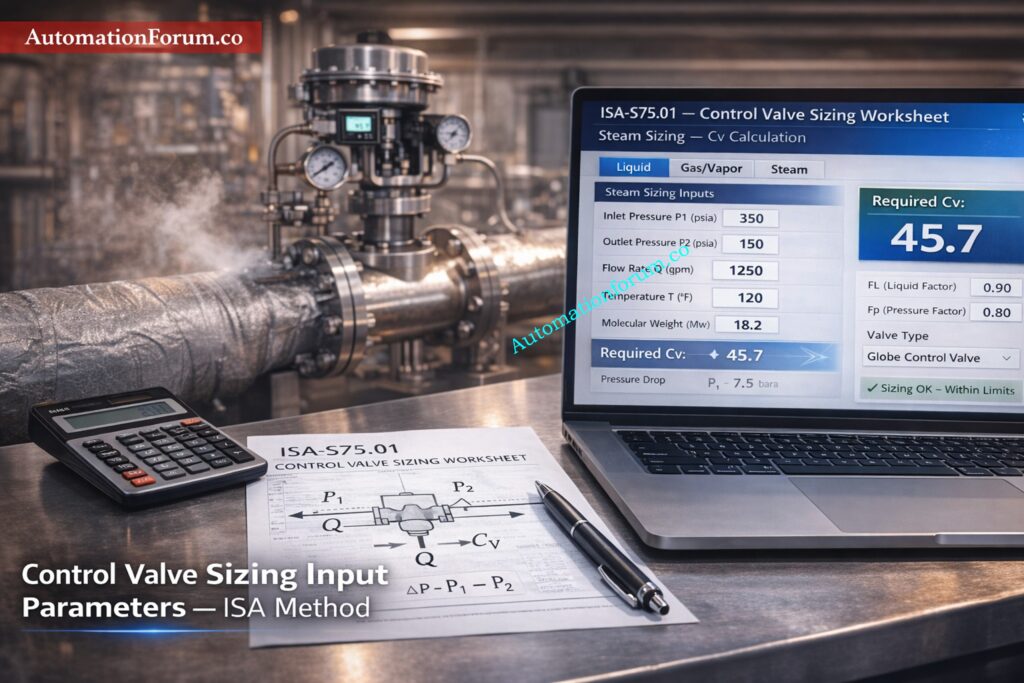
Using flow equations that take into account the needed flow rate, pressure drop, fluid characteristics, and Cv coefficient, the size of the control valve is determined. Engineers typically use IEC or ISA sizing formulas and vendor sizing software to determine the correct valve Cv and body size.
What are the Three Types Of Control Valves?
The three main types of control valves are Globe Valves, Ball Valves, and Butterfly Valves. Globe valves are preferred for precise control, ball valves for tight shutoff, and butterfly valves for large flow, low-pressure applications.
Refer the below link for Control Valve Noise Prediction Calculator – IEC 60534 Based Engineering Tool
automationforum.co·Your Trusted Source for Automation Power Tools & Solutions
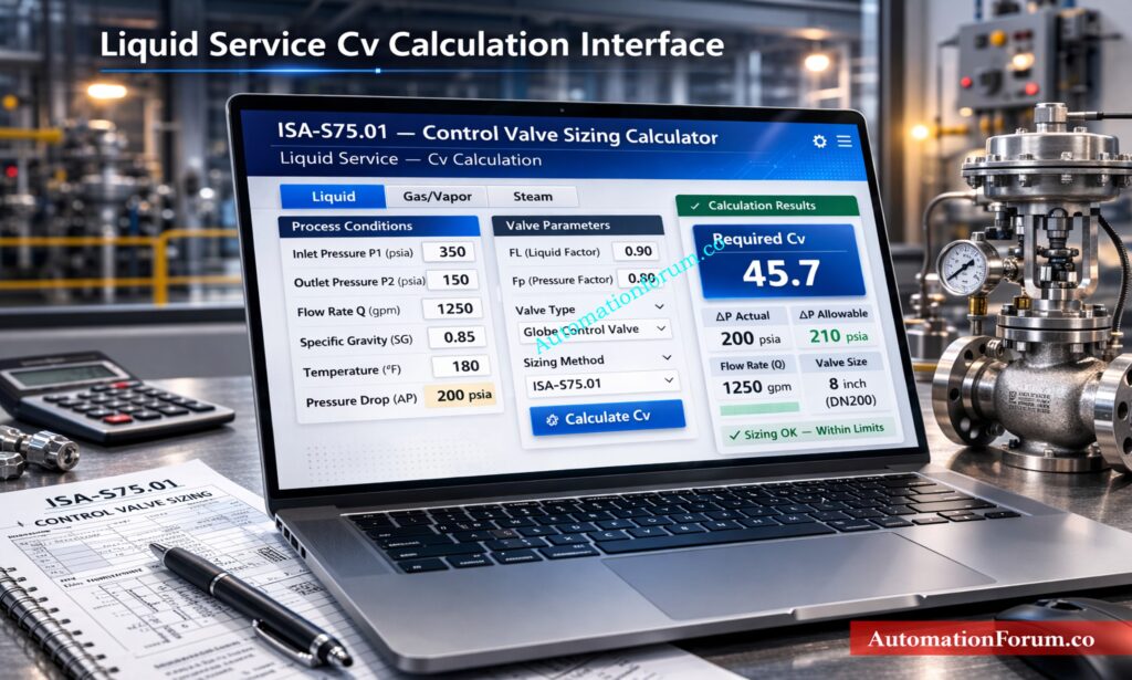
Control Valve Sizing Calculator and Why Correct Valve Sizing Matters
Control valves are the final control elements that have a direct effect on the safety, stability, and efficiency of a process. Proper size makes sure that flow management is correct, the loop works well, and the equipment lasts a long time. The control valve sizing calculator is an important tool for instrumentation engineers. It helps them figure out the Cv value they need based on things like pressure, temperature, flow rate, and fluid characteristics.
One of the most common mistakes engineers make while working on EPC projects and plant maintenance is not sizing valves correctly. A valve that is too small can’t supply the flow that is needed, which limits productivity and makes the process unstable. An oversized valve works close to the closed position, which makes it hard to control, generates oscillations, wears out the actuator too rapidly, and makes PID tuning unreliable.
If you size anything wrong, it could cause severe mechanical and operational problems, like:
A reliable control valve sizing calculator that follows the ANSI ISA valve sizing standard will help you acquire the proper valve and avoid costly failures.
What is Control Valve Cv? Definition, Units, and Flow Capacity Meaning
Cv, or flow coefficient, is the most significant number for sizing valves. It shows how much flow a valve can handle.
Definition:
A Cv is the amount of water that flows through a valve at 60°F and a pressure drop of 1 psi, measured in US gallons per minute.
Engineers can use this term as a standard reference to compare valves from different sizes and brands.
Physical Meaning
Cv is a measure of how easily fluid can pass through a valve. A higher Cv signifies a higher flow rate.
For instance:
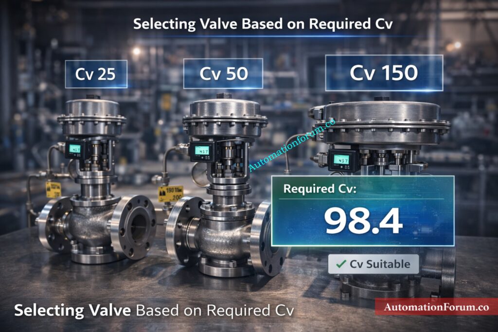
Cv = 1 → small flow capacity
Cv = 50 → medium flow capacity
Cv = 500 → large flow capacity
For each size and trim of valve, valve makers list the Cv values.
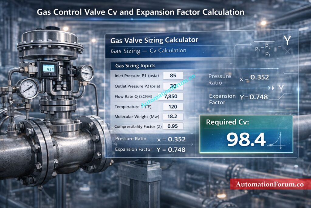
Control Valve Cv Formula Based on ISA S75.01 for Liquid, Gas, and Steam Applications
The simplified ISA S75.01 valve sizing equation for liquid service is:
Real-World EPC Engineering Tips for Accurate Control Valve Sizing
To avoid mixing up units, make sure that all projects use the same calculator template and that all units and N-constants are the same across the firm.
When making a data book, you should always run worst-case (min and max) flow scenarios through the calculator. Don’t only look at one point.
For valves that are very important for safety, use the calculator results along with vendor acceptance tests and make sure the purchase order includes performance guarantees.
Teach field maintenance crews how to spot the first signs of cavitation (such metallic rattling and louder noise) and keep extra trims on hand for quick replacement.
Control Valve Sizing Calculator: Frequently Asked Questions
How to size a control valve?
To get the right size for a control valve, you need to know the flow rate, upstream and downstream pressures, temperature, and characteristics of the fluid. Then you may use ISA S75.01 formulae to figure out the Cv. The valve you choose should let the most flow through while moving between 20% and 80% of the time. This makes sure that control stays stable and lasts a long time.
How is CV calculated?
Flow rate, pressure drop, and fluid specific gravity are used to figure out Cv. The usual formula for liquids is Cv = flow rate × √(specific gravity ÷ pressure drop). There are also correction factors for gas and steam, like expansion factor and compressibility.
What is the rule of thumb for control valve sizing?
Most of the time, you should choose a valve that opens between 20 and 80 percent of the way. Engineers also leave a Cv margin of 10% to 25% for future growth and dirt buildup. This stops things from getting too big and makes sure that control is accurate.
What is CV in control valve sizing?
Cv is the flow coefficient that shows how much fluid can flow through a valve when the pressure drops by a certain amount. It shows how much flow the valve can handle and is used to compare different sizes and trims of valves. A higher Cv signifies a larger flow capacity.
How to calculate Cv formula?
For liquids, Cv is the flow rate times the square root of the specific gravity divided by the pressure drop. When using the formula, all the units must be the same. When it comes to gas and steam, other things like temperature and pressure ratio are also taken into account.
What is a good Cv value?
A good Cv value is one that lets the valve work in the middle of its travel range while still meeting the highest flow rate. Usually, the Cv of the chosen valve is a little greater than the Cv that was estimated. This gives a safety margin and makes sure that process control stays stable.
Use ISA S75.01 And Control Valve Sizing Calculator To Avoid Failures
For safe and effective plant operation, it is important to size valves correctly. Engineers can use the control valve sizing calculator to correctly do the ISA S75.01 Cv calculation and choose the right valve for applications involving liquid gas and steam. It helps keep things from cavitating, flashing, choking, and becoming unstable, and it also makes process control and equipment life better. Instrumentation engineers can make sure that control valves work reliably, lower maintenance costs, and have the best process control throughout the plant’s life by using a control valve sizing calculator during design, commissioning, and maintenance.
Refer the below link for the Key Control Valve Performance Parameters Explained
Introduction to Solenoid Valve Troubleshooting in Process Industries
People who work with instrumentation in process sectors need to know how to fix solenoid valves. This difficult quiz is all about detecting electrical, pneumatic, and mechanical faults with solenoid-actuated valves that are utilised in the oil and gas, power, chemical, and industrial sectors. Engineers who work on maintaining instruments and automating factories will discover that the questions are mostly about root-cause analysis, field measurement techniques, diagnostic sequencing, and integrating control systems. Use real-life events to help you make better decisions in the plant, cut down on downtime, and make things safer and more reliable. This is a great test for control systems experts who want to see how well they can fix solenoid valves in a challenging, hands-on way. Finish it to show that you know what you’re doing and learn skills that will help you fix things in the field.
Advanced Solenoid Valve Troubleshooting Quiz – 25 Scenario-Based MCQs for Instrumentation & Control Professionals
Every EPC engineer that works in process industries needs to know a lot about HAZOP study instrumentation engineering. In complicated plants like oil and gas, petrochemical, chemical, and power plants, even a tiny change in pressure, temperature, or flow can have big effects on safety, the environment, and the economy. So, it’s important to know how HAZOP works and how its results affect the design of instruments. It is really important.
HAZOP is more than just a safety workshop for EPC engineers. It has a direct effect on the choice of instruments, the rationale behind alarms, the design of interlocks, the reasoning behind controls, and the plans for shutting down. When instrumentation is in line with HAZOP findings, the plant is safer, more dependable, and easier to run.
What is a HAZOP Study?
Definition and Core Principles of HAZOP
HAZOP is short for “Hazard and Operability Study.” It is a methodical and organized way to find possible dangers and problems with how a process plant works. The method looks at how things can go wrong with the design and what might happen as a result.
The main notion behind HAZOP is easy to understand. A team from different fields looks at the process in discrete parts called nodes. The team uses guidance words like More, Less, No, Reverse, and Other than to process characteristics like flow, pressure, temperature, and level for each node. These combinations create deviations, which are then looked at to find out what caused them, what happened as a result, and how to protect against them.
How HAZOP Differs from General Risk Assessment
HAZOP is far more thorough and scenario-based than a general risk assessment. It focuses on real-world process conditions and failures. That level of information makes it very useful for instrumentation engineering.
Why HAZOP is Critical for Instrumentation Engineering in EPC Work
Impact on Instrument Selection and Specification
Instrumentation is a key part of finding, controlling, and reducing the effects of deviations found in a HAZOP study. Most dangers in process plants only become serious when they aren’t found or controlled quickly enough. Sensors, transmitters, control valves, alarms, and shutdown systems are often the ones in charge of that.
For EPC engineers, HAZOP outcomes directly affect:
Selection of measurement technology
Accuracy and range of transmitters
Alarm set points and priorities
Safety instrumented functions
Cause and effect logic
Relationship Between HAZOP and Plant Operability
If HAZOP instructions aren’t followed well, the plant could have problems like false alarms, excursions that aren’t useful, or unsafe working conditions. In practice, having HAZOP findings and instrumentation design that are very similar makes things safer and more productive.
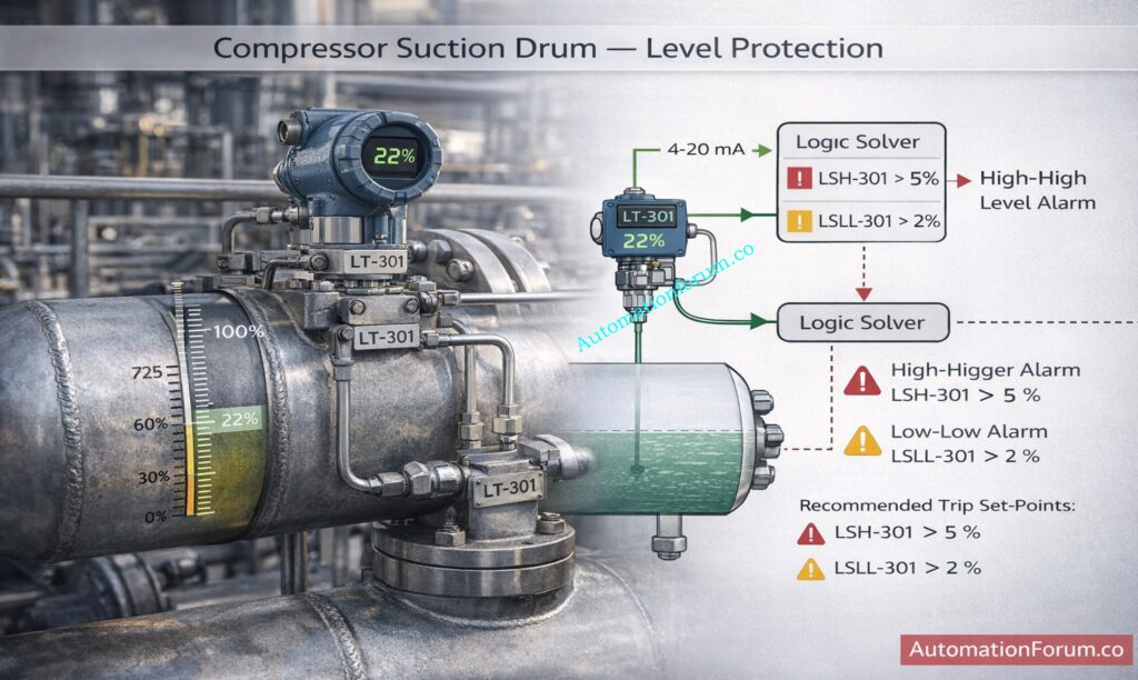
Case Study – Compressor Suction Drum HAZOP Analysis
Identifying More Level Deviation
Think about a node for the compressor’s suction drum. The goal of the design is to keep the pressure stable and stop fluids from getting to the compressor.
Instrumentation Safeguards and Trip Logic
The deviation More level is found during HAZOP. A level transmitter failure or a blocked output line could be the blame. The result might be liquid getting into the compressor, which could cause a lot of mechanical damage.
Implementation into Cause and Effect Matrix
A high-level alarm is a current protection. But the team thinks that the time it takes to respond to an alarm might not be enough. So, the suggestion is to add a high level trip that will turn off the compressor automatically.
After that, the instrumentation engineer needs to choose a dependable level transmitter, set points, update the cause and effect chart, and make sure that the shutdown logic is tested during commissioning.
Prioritizing and Closing HAZOP Actions in EPC Projects
Risk-Based Prioritization Strategy
Not every HAZOP action is equally risky. Instrumentation engineers must set priorities based on:
Severity of consequence
Likelihood of occurrence
Regulatory requirements
Project schedule constraints
Items that are very risky, like safety trips, need to be dealt with right away. Design optimization might include planning enhancements that lower risk.
Showing these materials clearly during HAZOP meetings makes the discussions better and lessens confusion.
Digital solutions like activity tracking systems and document management platforms assist make sure that suggestions don’t get lost between design stages.
Safety Integrity Level (SIL) and Safety Requirements Specification (SRS)
How HAZOP Drives SIL Determination
Safety Integrity Level (SIL) evaluation and a clear Safety Requirements Specification (SRS) are two important parts of HAZOP recommendations. If HAZOP finds a protective function that needs to work automatically, the instrumentation engineer has to decide if it should be a Safety Instrumented Function (SIF).
Converting Recommendations into Safety Instrumented Functions (SIF)
The SIF needs a clear SIL target that is based on the amount of risk that needs to be lowered. SIL allocation affects the choice of instruments, the voting architecture, diagnostics, and proof-test planning. The SRS should list the functional needs, types of input and output signals, response times that are expected, diagnostic coverage expectations, and proof-test intervals so that procurement and maintenance are in line with the HAZOP goal.
Refer the below link to Calculate SIL and Verify Safety Integrity Level Easily with our Online Calculator (IEC 61508 / 61511)
Testing, Commissioning, and Validation of HAZOP-Derived Functions
Factory Acceptance Test (FAT) Integration
Changes to the design that come from HAZOP are only useful if they are tested. Forced transmitter faults, impulse line blockage simulation, alarm annunciation tests, and trip response-time verification must all be part of Factory Acceptance Tests (FAT) and field loop inspections.
Site Acceptance Test (SAT) Verification
Site Acceptance Tests (SAT) and commissioning procedures must be able to mimic realistic deviations and keep track of the order in which events happen. Make test cases for each HAZOP activity and make sure that systems can be tested (for example, by adding test switches).
simulation points, and easy-to-reach test jacks, and save objective proof from FAT and SAT to show that each HAZOP-derived function works correctly in both normal and bad conditions. Only accept systems when the functions that come from HAZOP show that they work reliably.
HAZOP regularly points to warnings and manual operator actions as important safety measures. Technical safeguards can fail if alarms are poorly designed or if people anticipate them to work in ways that aren’t possible. Set up an alarm system that sorts alarms into groups, determines priorities, stops flooding, and organizes alerts that are connected to each other.
Operator Response Time Evaluation
Use HAZOP scenarios to run operator-in-loop simulations so that control room staff may practice emergency steps and diagnostic workflows. Give operators clear fast cards and checklists that list HAZOP-derived set points and activities, and plan regular drills to make sure people can do their jobs well when they are under stress.
HAZOP is an ongoing endeavor. Changes in engineering, capacity, or operating experience can make prior assumptions wrong. Plan targeted HAZOP revalidations following big changes, and keep a living HAZOP registry under document control so that changes automatically start risk reviews.
Managing Changes Through MOC Processes
Connect HAZOP activities to change management so that any changes to process conditions, software logic, or instrumentation must be assessed for risk before they are made. This lifecycle discipline keeps recorded assumptions from drifting away from what really happens in the field and helps keep safety measures working well throughout the life of the facility.
Regulatory Compliance, Audits and Documentation Traceability
Linking HAZOP Recommendations to Engineering Documents
In many places, you have to show that your instrumented protection systems meet regulations and that you have done a risk assessment. It is important to be able to trace things back: each HAZOP advice should be linked to datasheets, control narratives, cause-and-effect charts, SRS entries, FAT/SAT reports, and commissioning sign-offs.
Audit Evidence and Compliance Demonstration
This chain of evidence proves that something is in compliance during audits. Instrumentation engineers must regard HAZOP results as binding design inputs and guarantee that document control encompasses approvals, modification histories, and verification artifacts for each activity.
Cybersecurity Considerations in Modern Instrumentation HAZOP
Networked field devices, IIoT sensors, and remote diagnostics all raise cybersecurity issues that should be part of HAZOP’s scope. A fake communication channel or a sensor reading that has been changed can hide changes or induce trips that shouldn’t happen. When using digital instruments, make sure to include cybersecurity experts in HAZOP sessions. Set up secure protocols, authentication, encryption, and integrity checks for important measurement and command paths. Make sure that safety functions are somewhat separate from non-safety networks so that cyber attacks can’t turn off protective trips or alarms.
IIoT, Analytics and Predictive Maintenance Integration
Use data historians and analytics to check the assumptions made during the first operations of HAZOP. Trend analysis and anomaly detection can assist find instrument drift, sensor degradation, or strange process signatures before they become dangerous deviations. employ analytics to help with alarm rationalization, which will cut down on false alerts and help operators stay informed of what’s going on. Also, employ predictive maintenance tactics for important transmitters and actuators. When analytics back up HAZOP assumptions, they make the rationale for targeted spare parts and maintenance investments stronger.
Procurement and Vendor Management Based on HAZOP Findings
Use HAZOP-derived requirements to drive procurement specifications. Make sure that vendors give you FAT evidence, loop designs, proof-test protocols, and calibration certificates for safety devices. Include HAZOP action close-out as a contract milestone and let vendors take part in FAT scenarios. To cut down on downtime, make a plan for spare parts for important parts, such as calibrated hot spares, repair kits, and clear policies on when to fix and when to replace. Include warranty and support terms that say the seller must help you quickly with any issues that influence safety functions. Well-written handover documents and training during vendor handover make sure that operations have both the hardware and the knowledge they need to keep HAZOP-required safety measures in place.
Governance, KPIs and Accountability for HAZOP Closure
Set up explicit rules for closing HAZOP actions by giving responsible owners, setting reasonable timeframes, and include HAZOP actions in project and maintenance KPIs. Use a verification trace matrix to keep track of how close you are to closing, and if safety items are overdue, tell the steering committees. Use KPI dashboards that display alarm rates, proof-test completion, spare parts availability, and the average time it takes to fix important transmitters. Link maintenance budgets and spare parts planning to risk priorities that come from HAZOP so that funding goes to the biggest risk reductions. This governance makes ensuring that HAZOP recommendations turn into measurable results instead of just sitting in a report.
Continuous Improvement and Lessons Learned from HAZOP Implementation
Post-Commissioning Review
Embed learning loops. After commissioning and during early operations, track incidents, alarms, and maintenance trends against HAZOP expectations. Where gaps appear, analyze root causes and feed lessons back into design standards, procurement specs, and future HAZOP sessions. Metrics such as alarm rate per operator, trip cause distribution, and mean time between failures for critical transmitters help prioritize improvements and justify investments in redundancy or upgrades. A data-driven feedback loop makes HAZOP a practical, evolving tool that continually reduces operational risk.
Feedback into Future EPC Projects
For EPC engineers that work in process industries, HAZOP study is much more than just a legal necessity. It is a useful engineering tool that directly affects the design of equipment, the way alarms work, and the rationale behind shutting down. The plant is safer, more reliable, and easier to operate when instrumentation engineers are involved, understand deviations well, and make sure that everyone follows through.
Building a Risk-Aware Engineering Culture
In the end, a solid connection between HAZOP findings and instrumentation engineering turns theoretical risk analysis into real-world safety.
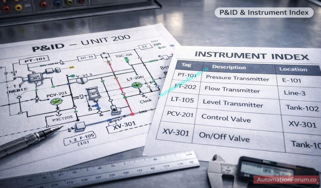
What Documents Should Instrumentation Engineers Bring to a HAZOP?
Instrumentation engineers should have the latest P&IDs, instrument index, cause-and-effect matrix, control narratives, and alarm philosophy papers with them.
They also need to check datasheets, SIL studies (if they exist), and loop diagrams to make sure that the talks are technically correct..
When Should a HAZOP Recommendation Become a SIF?
A HAZOP suggestion turns into a Safety Instrumented Function (SIF) when an automatic action is needed to lower the risk to an acceptable level.
If operator response or basic control systems aren’t good enough, a SIL-assessed SIF must be put in place.
How Often Should HAZOP Be Revalidated?
After making big changes to the process, control, or capacity, HAZOP should be revalidated.
Every five years, or as needed by company or regulatory norms, periodic revalidation is usually done.
What Is the Role of EPC Engineers in HAZOP Action Closure?
EPC engineers are in charge of turning HAZOP suggestions into new design documents and plans for putting them into action.
Why Noise and Signal Stability Matter for Instrumentation DCS and Product Quality
In process industries the ability to observe and interpret noise and signal stability during running inspection is not optional it is essential.
Proper noise and signal stability observation ensures that process variable readings are reliable and that control actions taken by the distributed control system are appropriate.
When instrument signal noise goes unnoticed or when signal instability persists it can lead to control loop hunting and repeated corrective actions that do not address the root cause.
This creates poor product quality increased downtime and excessive maintenance work orders. For field instrumentation and control engineers practical observability techniques tied to DCS PV trend analysis enable fast diagnosis of electrical and loop tuning problems.
A disciplined approach to signal inspection reduces nuisance alarms in DCS and prevents slow creeping faults from becoming safety incidents.
This article gives instrumentation and control engineers a field oriented guide to recognizing electrical noise patterns differentiating them from control tuning issues and applying inspection and corrective measures that keep process control stable and predictable.
Understanding Noise and Signal Instability in Instrumentation
What is Instrument Signal Noise and its Causes
Signal noise in instrumentation refers to unwanted variations superimposed on the true measurement of a process variable.
Noise may be random short duration spikes it may be narrow band ripple at a specific frequency or it may be partly periodic oscillation that looks like low frequency ripple.
Instrument signal noise can come from wiring faults electromagnetic interference from motors or variable frequency drives ground loops or degraded power supplies.
Signal instability on the other hand refers to variations in the measured process variable that are persistent and may change slowly or in cycles.
Instability can be caused by sensor mechanical looseness poor mounting process disturbances or by control system feedback issues.
An unstable process variable has direct consequences for the DCS. If the DCS reads a fluctuating PV it will calculate corrective moves that in turn change the manipulated variable.
If that corrective action is too aggressive given the process dynamics control loop hunting can start. Control loop hunting is the repeated overshoot and recovery cycle that wears mechanical components accelerates valve and actuator failure and degrades control performance.
Persistent instrument signal noise increases the frequency of nuisance alarms in DCS and reduces operator trust in displays and trending.
For these reasons noise and signal stability observation should be part of every running inspection and every loop troubleshooting exercise.
How Noise and Signal Instability Affect DCS Performance and Control Loop Hunting
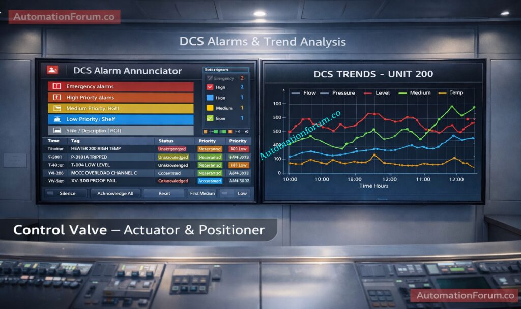
Observing Process Variable PV Trends on the DCS
DCS PV trend analysis is the frontline tool for field engineers during running inspection. A well configured PV trend shows the true behavior of a process variable across time and allows the engineer to separate random spikes from oscillation and ripple.
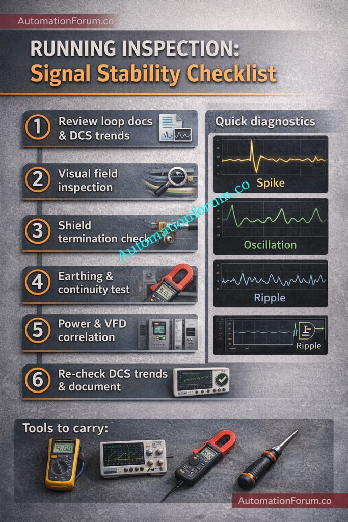
Identifying Random Spikes in Process Variable Trends
Random spikes are single or isolated excursions that return to baseline quickly. They often appear on PV trends as thin sharp peaks.
Common causes include loose wiring at terminal blocks poor shield termination intermittent connector contact and transient electromagnetic pulses from nearby switching equipment.
Power supply disturbances or battery backed devices entering a diagnostic state can also create spikes.
On the trend a spike will not necessarily repeat at a fixed frequency and will often coincide with mechanical activity or personnel work near the cable route.
During shield termination inspection check for loose crimps broken conductor strands or signs of moisture ingress that create intermittent contact.
Oscillation appears on trends as a repeating up and down cycle. The frequency may be slow or fast depending on the loop dynamics.
Process variable oscillation can indicate control tuning that is too aggressive feedback delay introduced by slow sensors or valves with sticking behavior.
Noisy input can confuse the controller and amplify oscillation.
Distinguishing tuning induced oscillation from electrical noise requires correlating the PV trend with the controller output trend and the final control element trend.
If the controller output mirrors the PV oscillation and valve travel is substantial then tuning is likely involved.
If the valve is static but the PV oscillates the issue is likely upstream in sensing or process flow.
Ripple is high frequency periodic variation on the PV trace. On the trend it appears as a thin band of rapid movement around the baseline.
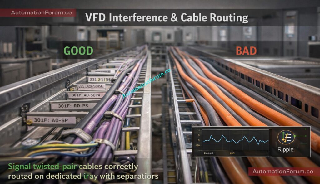
Ripple is commonly caused by VFD interference in instrumentation or power cable induction when signal and power cables run together.
Ripple often has a consistent amplitude and frequency tied to the switching frequency of nearby drives.
When ripple is present inspect cable routing and power electronics near the sensor and apply shield termination inspection and earthing inspection techniques to mitigate.
Practical DCS PV trend analysis techniques include using zoom and time compression tools to view both macro and micro behavior comparing PV trend with controller output and valve position overlaying digital status signals such as VFD running and comparing trends across redundant sensors.
Export short trend segments for offline analysis when needed. Use trend annotations to mark inspection times and observed events so later root cause analysis is simpler.
Step by Step Running Inspection Procedure for Signal Stability
A step by step running inspection is central to maintaining reliable signal transmission. Follow each step with both purpose and the technical reasoning in mind.
Preparation Before Field Visit and Documentation Review
Get the right work permit and work with operations if you need to launch or close a business.
Purpose: Make sure the inspection is safe and focused. Technical Reasoning: Understanding loop behavior before touching wiring avoids unnecessary disturbance and speeds root cause identification.
Visual Field Inspection of Cables Junction Boxes and Conduits
Walk down the complete signal path: instrument → junction box → cable tray → marshalling panel.
Check the junction boxes, cable trays, conduits, and glands.
Check for broken wires, damaged insulation, loose glands, open conduit entrances, and moisture getting in.
Find temporary fixes like taped joints or wires that are out in the open.
Purpose: Find out what physical and environmental factors are making the signal unstable. Technical Reasoning: Mechanical strain and moisture break down insulation and shielding, which might cause noise or signal drift to happen from time to time.
Refer the below link for the How to simulate 4-20ma signal with Loop Calibrator ?
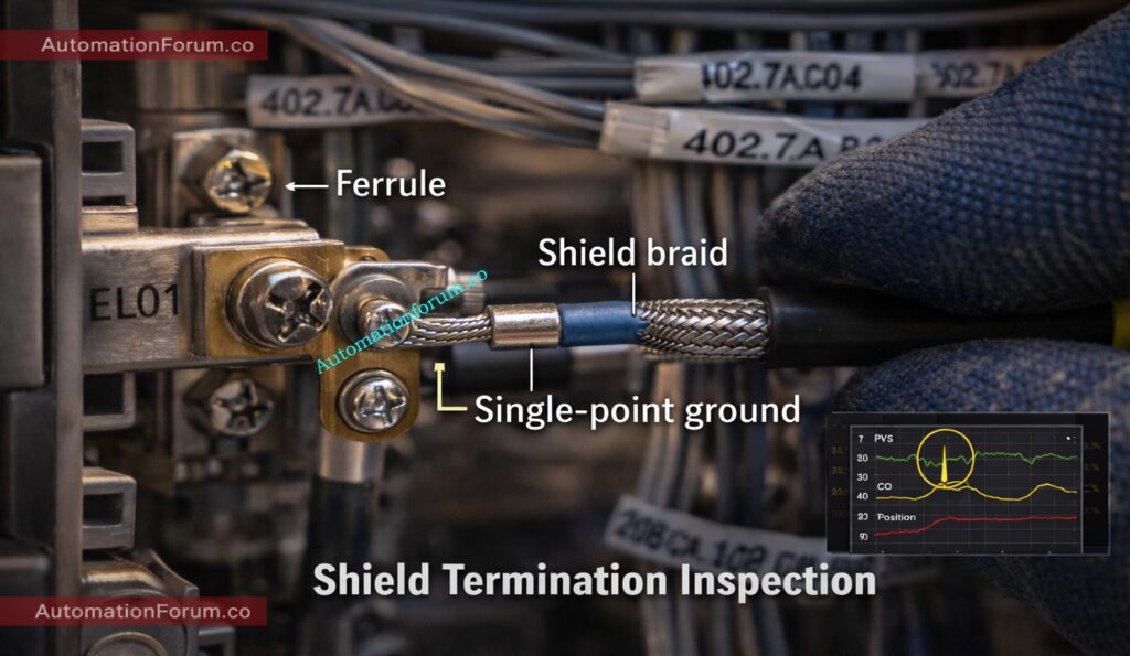
Make sure that the cable shield is continuous and appropriately terminated.
Check that the way the termination is done fits the plant’s standard (usually single-point grounding at the panel side unless the vendor says different).
Check that the shield braid isn’t wrapped around the signal wires.
Check that the ferrules and crimping are correct.
Purpose: Prevent electromagnetic interference (EMI). Technical Reasoning: If the shield termination is wrong, outside electromagnetic fields can get into signal cores, which might cause spikes or ripples.
Earthing Inspection and Ground Integrity Verification
Check the connections between the instrument’s earth and the panel’s earth.
Tighten the bonding points and get rid of any rust that may be there.
Use an earth clamp meter to check for continuity in the ground.
Check that the resistivity of the earth satisfies the plant’s standards.
Purpose: Keep the reference potential steady. Technical Reasoning: Bad earthing makes the ground potential different, which shows up as noise, offset, or unstable PV measurements.
Look for more than one grounding point on the body of the shield or instrument.
If possible, temporarily separate the secondary grounding point and watch the DCS trend.
Reconnect right after the test.
Purpose: Find unwanted currents that are flowing. Technical Reasoning: Ground loops cause sluggish drifting signals or low-frequency oscillations because there are minor voltage changes between earth points.
Cable Routing Verification and Separation from Power Cables
Make sure that power and motor wires are not touching signal cables.
Look for large runs of high-current wires that are parallel.
Check to see if there are tray separators if you have to share a tray.
Purpose: Lower electromagnetic coupling. Technical Reasoning: Long parallel routing increases inductive and capacitive coupling, especially from VFD driven motors.
Inspection of Nearby VFD Panels and High Power Equipment
Find VFD panels, motors, transformers, or switching equipment that are close by..
Correlate PV fluctuations with motor start/stop or load changes.
Check the distance between the tray and the cable crossings.
Purpose: Find sources of EMI that happen from time to time. Technical Reasoning: When VFDs switch frequencies, they add high-frequency noise to analog signals, which might look like ripples or repetitive spikes.
Power Supply Quality and DC Ripple Measurement
Check the DC voltage going to the transmitter.
Use a multimeter (AC range) or an oscilloscope to look for AC ripple.
Check the readings against the limits set by the manufacturer.
Purpose: Make sure the supplied voltage to the transmitter stays steady. Technical Reasoning: Excessive ripple on 24 VDC supply modulates transmitter electronics, resulting in noisy or unstable output signals.
Open junction boxes and panel terminals (with permit).
Inspect for loose screws, discoloration, overheating, or corrosion.
Tighten the terminals to the right amount of torque.
Clean corroded contacts and apply contact protection if required.
Purpose: Get rid of spots of resistance that come and go. Technical Reasoning: Terminals that are loose or corroded cause contact resistance to change, which causes spikes and signal drops.
Insulation Resistance and Continuity Testing
If the technique allows it, do an insulating resistance test.
Check conductor continuity end-to-end.
Check that the polarity is accurate and that there are no shorts.
Purpose: Find hidden damage to cables. Technical Reasoning: Low insulation resistance or partial shorts cause leakage currents that mess up low-level analog signals.
Instrument Head Inspection and Configuration Verification
Look for water inside the transmitter housing.
Check that the cable gland is tight and sealed.
Check that the settings for range, zero, and damping are right.
If necessary, use a calibrator to check the function.
Purpose: Make sure the transmitter is working properly and is set up correctly. Technical Reasoning: Moisture inside the transmitter, a wrong setup, or loose terminals can make it seem like there are noise problems outside.
Watch for changes in spikes, oscillation, or ripples.
Confirm improvement after corrective action.
Purpose: Establish cause-and-effect validation. Technical Reasoning: Real-time trend improvement verifies the true origin of the issue and averts unnecessary alterations.
Maintaining Signal Integrity to Prevent Loop Hunting and Nuisance Alarms
Noise and signal stability observation during running inspection is a useful talent that combines rigorous DCS PV trend monitoring, field inspection, and targeted electrical diagnostics. Identifying random spikes oscillation and ripple on trend traces and then applying systematic inspection steps such as shield termination inspection earthing inspection and power ripple checking reduces control loop hunting and cuts down nuisance alarms in DCS. Using the right tools at the right time and following sound grounding and cable routing practices yields stable reliable signals and a more robust control system.
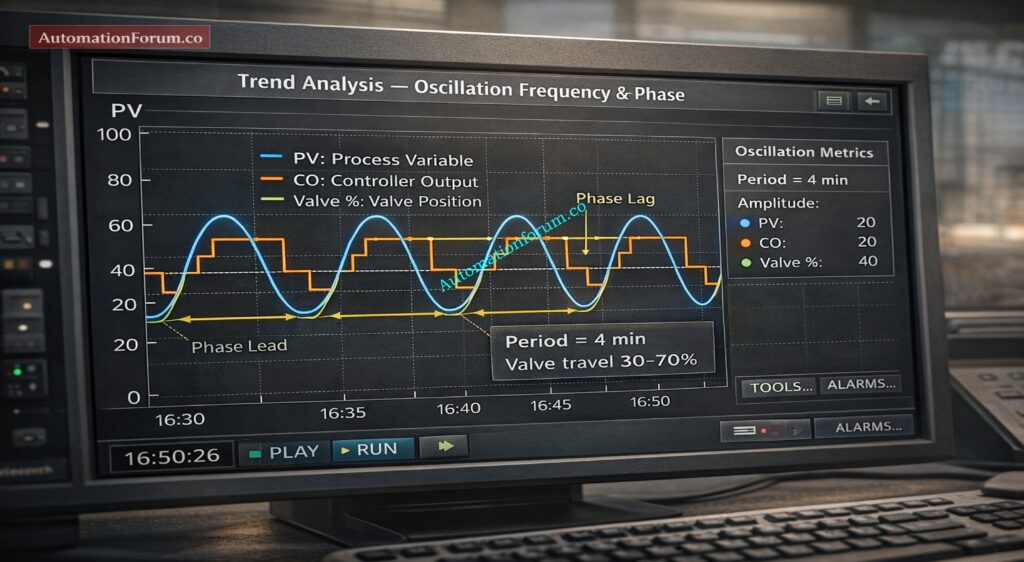
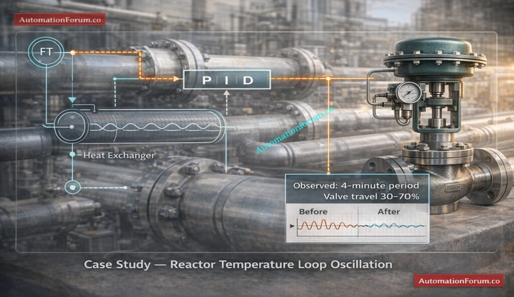
Introduction to Control Valve Hunting Due to PID Controller in Industrial Process Control Systems
Why Troubleshooting Control Valve Hunting Is Critical for Instrumentation, Control and Maintenance Engineers in Oil and Gas, Petrochemical and Power Plants
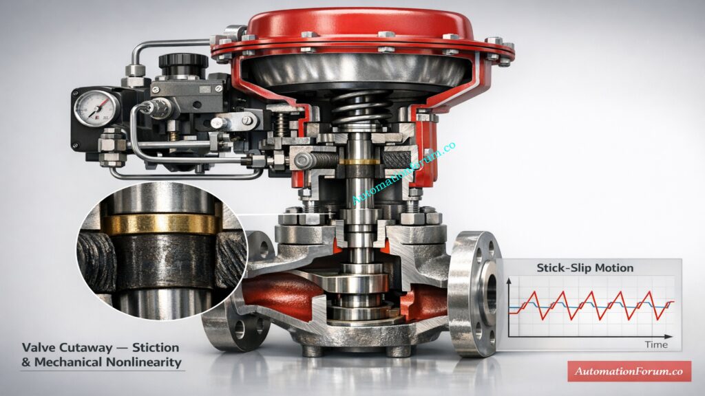
In industrial process control systems, control valve hunting caused by PID controllers is a frequent yet serious issue. It happens when a control valve doesn’t smoothly stabilize but instead oscillates around the setpoint continuously. This repeated oscillation is typically caused by improper PID tuning, excessive controller gain, process dead time, valve mechanical issues, or loop interaction.
In oil and gas, petrochemical, and power plant industries, unstable loops directly affect product quality, energy efficiency, equipment life, and operational safety. Instrumentation engineers and technicians in charge of plant dependability and process stability must comprehend the underlying reasons of control valve hunting caused by PID controllers and employ a systematic troubleshooting method.
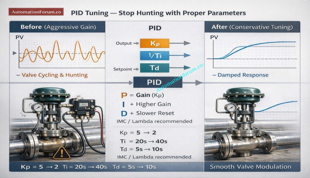
How to Use This Step-by-Step PID Tuning and Control Valve Hunting Troubleshooting Guide to Restore Loop Stability and Prevent Valve Oscillation
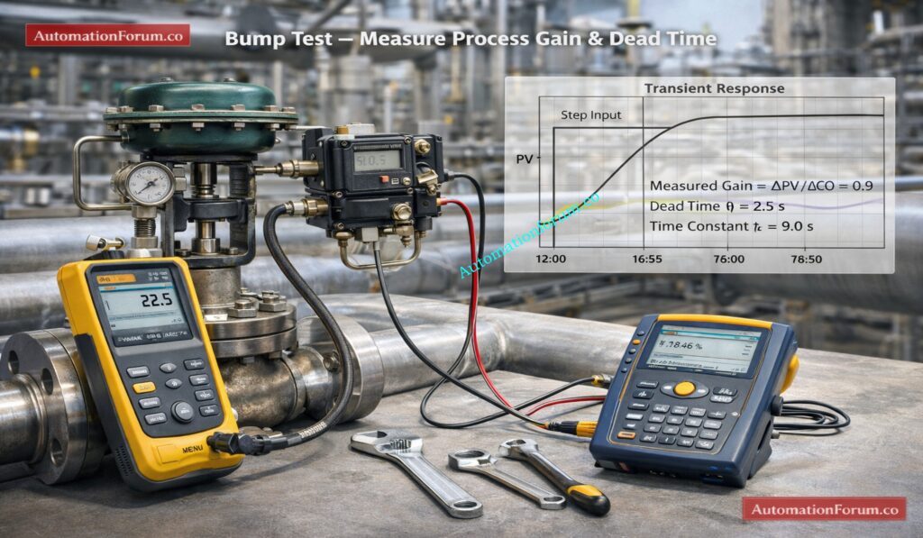
In any closed loop control system, the objective is simple. Maintain the process variable at the desired setpoint with minimal deviation and smooth actuator movement. When the PID parameters are incorrectly adjusted, the controller may react too aggressively or too slowly, causing the loop to become unstable.
Instead of correcting disturbances smoothly, the system overshoots, reverses, and repeats the cycle. The valve continuously moves back and forth, creating a condition known as hunting. This tendency eventually leads to operator annoyance, increased actuator stress, and damage to valve components.
What Is Control Valve Hunting in a Process Control System?
Technical Definition of Control Valve Hunting in PID-Based Closed Loop Systems
One frequent instability issue in industrial process control systems is control valve hunting. It describes a control valve’s prolonged cyclic movement combined with the process variable’s (PV) ongoing oscillation. The method overshoots and undershoots the desired value because the valve continually opens and closes in a rhythmic manner rather than gradually regulating to maintain setpoint.
How Control Valve Hunting Appears in DCS and PLC Trend Analysis
One frequent instability issue in industrial process control systems is control valve hunting. It describes a control valve’s prolonged cyclic movement combined with the process variable’s (PV) ongoing oscillation. The method overshoots and undershoots the desired value because the valve continually opens and closes in a rhythmic manner rather than gradually regulating to maintain setpoint.
Hunting is a sign of an improperly balanced feedback control loop from the standpoint of instrumentation and control. Poor PID tuning, high controller gain, integral windup, dead time, valve stiction, actuator problems, or signal noise could all be contributing factors. Control valve hunting must be recognized and addressed in order to preserve dependable plant operation and increase valve service life.
Difference Between Normal Control Valve Modulation and Control Valve Hunting
Field engineers, loop tuning experts, and maintenance teams must be able to distinguish between healthy control action and unstable oscillation.
Characteristics of Stable Control Valve Modulation in Properly Tuned PID Loops
The valve exhibits predictable behavior in a control loop that is steady and appropriately adjusted:
Small, smooth valve movement
Quick settling after a disturbance
Minimal overshoot
Stable process variable
Damped response over time
Gradual correction toward setpoint
In this case, the process variable converges toward the setpoint without constant cycling while the controller output gradually changes. This indicates good loop tuning and proper interaction between controller, final control element, and process dynamics.
Warning Signs and Oscillation Patterns of Control Valve Hunting in Industrial Automation Systems
On the other hand, there are obvious indications of instability in control valve hunting:
Repetitive oscillation
Noticeable overshoot and undershoot
Regular periodic waveform on trend
No natural damping
Continuous valve travel swings
Increased mechanical stress on actuator and trim
In the DCS or PLC trend, the oscillations usually happen at regular intervals and produce a sinusoidal or repeating pattern. If corrective action is not taken, the amplitude can stay the same or even rise.
Practical Example of Control Valve Hunting in a Heat Exchanger Temperature Control Loop
Oscillation Pattern, Valve Travel Fluctuation and Process Impact
Consider a heat exchanger temperature control loop in a process plant. If the outlet temperature oscillates every three minutes and the valve travel swings repeatedly between 40 percent and 65 percent, the loop is clearly unstable.
Operational and Maintenance Consequences of Sustained Valve Oscillation
Instead of stabilizing near the setpoint, the controller continuously overcorrects. In an established cycle, the temperature rises over the setpoint and subsequently falls below it. This state speeds up wear on the actuator diaphragm, stem, and control valve packing while also increasing energy consumption and decreasing heat transfer efficiency.
Persistent hunting can result in production losses, subpar products, and higher maintenance costs in major process sectors including petrochemical, oil and gas, and power generation facilities.
Early hunting detection through trend analysis and loop performance monitoring is crucial for instrumentation engineers and control system specialists. Oscillations can be avoided and steady performance restored with the aid of proper PID tuning, valve maintenance, and signal integrity checks.
How PID Controller Settings Cause Control Valve Hunting and Loop Instability
The most popular control algorithm in industrial process control systems is a PID (Proportional Integral Derivative) controller. Control valve hunting can be directly caused by aggressive tuning parameters or faulty configuration, even if it offers precise and reliable control when adjusted correctly.
Understanding Proportional, Integral and Derivative Action in Process Control
Three control terms are used by the PID controller to determine its output:
Proportional reacts to present error
Integral reacts to accumulated past error
Derivative reacts to rate of change
The feedback control loop becomes unstable when these three terms are not appropriately balanced. This instability manifests as hunting, which is the recurrent movement of the control valve and prolonged oscillation of the process variable.
Inadequate PID tuning causes the control system to oscillate continuously, disrupts loop balance, and decreases stability margins.
Effect of Excessive Proportional Gain on Valve Oscillation
The controller’s response to the present error between the setpoint and process variable is determined by proportional gain.
When the proportionate gain is excessively high:
Small error produces large output change
Process overshoots setpoint
Error reverses sign
Controller reacts strongly again
Continuous oscillation develops
Control valves exhibit fluctuating behavior as a result of this frequent error reversal. The valve keeps moving back and forth instead of settling at a stable position.
In processes with significant dead time, such as temperature loops in heat exchangers or long pipeline flow systems, high proportional gain drastically reduces phase margin. When phase margin decreases, loop stability is compromised, and sustained oscillation begins. Excessive gain makes the controller overly sensitive, turning minor disturbances into major control actions.
Integral Windup and Aggressive Integral Action as a Cause of Hunting
Integral action eliminates steady state error by accumulating error over time. This is necessary for precise control, but aggressive integral values can quickly make the loop unstable.
If integral time is too short:
Integral accumulates too quickly
Overshoot increases
Integral windup occurs
Oscillation continues without damping
Aggressive integral action is a big cause of PID tuning issues in sluggish processes like level control in tanks or big thermal systems. The controller keeps adding error even after the valve has reached its maximum, which means that corrective action takes longer and is too much.
The integral term can push the valve well beyond of the stable functioning range if it doesn’t have the right anti-windup protection, which can cause hunting to happen all the time.
Derivative Action and Noise Amplification in Industrial Signals
By predicting the future trend of error, derivative action creates damping. It responds to how quickly the process variable is changing, and when used effectively, it can make things more stable.
But derivative action also makes measurement noise worse.
If there is electrical noise or process problems in the transmitter signal:
Derivative term creates output jitter
Valve moves rapidly in small increments
Small oscillations grow over time
Mechanical wear increases
In real-world industrial settings, signals that are too loud are typical because of grounding problems, interference, or sensor wear. If you don’t filter properly, using derivative action can make valve oscillations worse instead of better.
You should only use derivative control when the signal quality is high and the signal is adequately filtered.
Wrong PID Mode Selection (Direct vs Reverse Acting) and Configuration Errors
If you set up the PID wrong, it might turn a stable loop into an unstable one right away.
Choosing the wrong control action is a common mistake:
Direct acting instead of reverse acting
Reverse acting instead of direct acting
This design mistake makes positive feedback instead of negative feedback, which makes things unstable right away and leads the control valve to hunt quickly.
Some such mistakes in the configuration are:
Disabled anti-windup protection
Incorrect output limits
Improper cascade tuning
Wrong sampling time
Incorrect scaling of input signal
These misconfigurations directly cause oscillations in process control systems that are caused by PID controllers.
Loop Interaction and Cascade Control Instability
Control loops in factories don’t usually work on their own. It’s common for multiple loops to affect each other, and instability in one loop might spread to another.
For instance:
Flow loop aggressively tuned
Temperature loop depends on flow
Flow oscillation transfers instability
Temperature valve begins hunting
When diagnosing valve oscillation, you should always check loop interaction. Bad tuning of the cascade, response times that don’t match, or control mechanisms that don’t agree with each other can make the system more unstable.
Understanding process dynamics and ensuring proper coordination between loops is essential to prevent control valve hunting.
Poorly tuned PID controllers frequently trigger control valve hunting by introducing excessive corrective action and reducing phase margin. To prevent oscillation, engineers should follow systematic PID tuning procedures, verify process dead time, and start with conservative gain settings.
Recommended practices include:
Implementing anti-windup protection
Applying derivative filtering
Setting proper output limits
Performing loop performance analysis
Checking valve stiction and actuator response
Verifying transmitter signal quality
Before making changes to live processes, simulation tools, loop tuning software, and performance monitoring systems can help find safe tuning settings.
In industrial automation systems, keeping the signal clean, making sure the valves are working properly, and using balanced PID tuning all make the loop more stable, decrease wear and tear on the machinery, improve the quality of the products, and make the whole process more efficient.
Common Signs of Control Valve Hunting Due to Improper PID Tuning
You can find control valve hunting caused by bad PID tuning by carefully looking at trends and observing the field. Instrumentation engineers can stop catastrophic process instability and equipment damage by spotting these warning indicators early.
Persistent sinusoidal trend pattern
Valve position oscillates regularly
Controller output oscillates at the same frequency
Process variable does not settle at setpoint
Frequent operator intervention required
Audible actuator cycling or repetitive mechanical noise
Understanding trends is important. If the valve position always comes before the process variable, the controller is probably causing the oscillation instead than responding to a process disruption.
DCS trend monitoring and loop performance analysis can help find problems early, which makes control systems more reliable, cuts down on maintenance costs, and keeps industrial processes running smoothly.
These things mess up the loop’s dynamics and make it less stable overall.
Process Dead Time and Phase Margin Reduction in Feedback Control Loops
In the control loop, dead time causes a lot of phase lag. More phase lag means less phase margin, and less phase margin means that oscillation will continue.
The PID controller keeps responding to old error data when the process reaction is delayed. Because of this delayed correction, there are recurrent overshoots and undershoots, which leads to constant valve hunting and unstable process variable behavior.
Valve Stiction, Backlash and Mechanical Nonlinearity Effects
One of the most common mechanical reasons for PID tuning issues is valve stiction.
Valve sticks due to friction
Controller output increases gradually
Valve suddenly jumps to a new position
Overshoot occurs
Cycle repeats continuously
This stick-slip behavior makes the final control element respond in a way that isn’t linear. Mechanical nonlinearity makes bad PID tuning worse, making loops that are only slightly tuned unstable.
Taking care of the valves, making up for dead time, and tuning the loop in a methodical way all help to prevent valve oscillation and make the process control performance and operational efficiency much better.
Step-by-Step Troubleshooting Guide to Stop Control Valve Hunting
Step 1: Analyze High-Resolution Trend Data and Identify Oscillation Frequency
Get data with a lot of detail. Find the period and amplitude of the oscillation. Look at the phase relationship between the valve and the process variable..
Step 2: Verify PID Parameters and Compare with Commissioning Values
Write down the proportionate gain, the integral time, and the derivative time. Look at the original commissioning values.
Step 3: Inspect Control Valve Mechanical Condition and Check for Stiction
Do a stroke test. Look for reaction and stiction. Check how well the positioner works.
Step 4: Perform Bump Test to Measure Process Gain, Time Constant and Dead Time
Make a modest adjustment to the output. How to Measure:
Process gain
Time constant
Dead time
For correct PID parameter modification, these values are needed.
Refer the below link for the What is Partial Stroke Test (PST)? A Complete Guide for Shutdown and Control Valves
Real World Case Study of Control Valve Hunting Due to Improper PID Tuning in a Petrochemical Reactor
After the feed composition changed, the temperature control loop in a petrochemical reactor started to oscillate. The disturbance altered process dynamics, but the existing PID tuning parameters were not adjusted accordingly. As a result, the control valve started hunting, causing instability and product quality variation.
Observed Oscillation Behavior and Trend Analysis
Four-minute oscillation cycle
Valve movement from 30 percent to 70 percent
Product quality deviation
Increased operator monitoring
The DCS trend showed a clear sinusoidal waveform, confirming sustained oscillation rather than random disturbance.
Root Cause Diagnosis Including Dead Time and Aggressive PID Parameters
A detailed investigation of the loop showed:
Dead time: 40 seconds
Time constant: 150 seconds
High proportional gain
Short integral time
Minor valve stiction
The large proportional gain and short integral time made the phase margin much smaller. Dead time made instability much worse, and slight valve stiction made oscillatory behavior even worse.
Corrective Actions Applied to Restore Loop Stability
A methodical way to fix problems was used:
Reduce proportional gain by 40 percent
Increase integral time
Disable derivative action
Service and lubricate control valve
Measured Improvement in Process Stability and Product Quality
Frequently Asked Questions About Control Valve Hunting and PID Tuning Problems
What is the cause of control valve hunting
Improper PID tuning, like high proportional gain or aggressive integral action, is what mostly causes control valve hunting. It can also result from process dead time, valve stiction, signal noise, or loop interaction that makes the controller overcorrect continuously.
What Is the Most Common PID Parameter That Causes Control Valve Hunting
Excessive proportional gain is the most common PID parameter that causes hunting. When gain is too high the controller reacts too aggressively to small errors and creates sustained oscillations in the valve and process variable.
What is hunting in controls
Hunting in controls is a condition where the control system continuously oscillates around the setpoint instead of stabilizing. The process variable repeatedly overshoots and undershoots, forming a regular waveform in trend data.
How Can I Differentiate Between Valve Stiction and PID Tuning Problems
When a valve sticks, the controller output normally has a sawtooth pattern, and the valve position suddenly jumps. PID tuning problems usually show smooth sinusoidal oscillations when the process variable follows the controller output.
Should Derivative Action Be Used to Stop Valve Hunting
Derivative action can help add damping and improve stability in some loops. However it can amplify signal noise, so it should only be used when measurement signals are clean and properly filtered.
How to Achieve Long-Term Loop Stability and Eliminate Control Valve Hunting in Industrial Automation Systems
Control valve hunting produced by a PID controller is basically a problem with the stability of the control loop. This might happen because the PID tuning is wrong, there is too much dead time, there are mechanical flaws, or the loops interact with each other. A organized troubleshooting procedure that includes trend analysis, bump testing, mechanical inspection, and improved PID tuning makes sure that processes stay stable over time, use less energy, and work reliably in industrial automation.
Proper PID parameter adjustment combined with correct valve sizing and preventive maintenance ensures stable process control, longer equipment life, improved product quality, and enhanced plant reliability.
Introduction to Dry Calibration of Displacer Level Transmitters
In the oil and gas, petrochemical, refinery, chemical, and power plant industries, dry calibration of a displacer-type level transmitter, often known as a Level Troll, is a regular part of commissioning and maintenance. The calibration is done by mimicking buoyancy using computed weight loss data instead of actually filling the container with liquid.
Who this Guide is For
This approach is used a lot in EPC projects where process liquid might not be accessible before commissioning. A solid Level Troll Weight Loss Calculator makes sure that the results are correct and can be repeated without making mistakes in calculation by hand.
In this complete guide, you will learn:
The working principle of displacer level transmitters
This article is structured for instrumentation engineers, control engineers, DCS engineers, and commissioning professionals working in process industries.
Trusted Resource for Instrumentation & Automation Engineers
ISA-5.1IEC 60751API 5.6
Level Measurement · Displacer Type
Level Troll Weight Loss Calculator
A precise engineering tool for dry calibration of displacer-type
level transmitters. Compute buoyancy weight loss, LRV / URV calibration weights
& full 4–20 mA linearity check values — no process liquid needed.
⚠ Please enter valid positive values in all fields.
📦
—
Volume (cm³)
⚖️
—
Weight Loss
🎯
—
100% Cal. Weight
📊 Dry Calibration Points (4–20 mA)
Level %
Signal
Cal. Weight
Tag
Description
Step-by-Step Working
💡 How Dry Calibration Works
A Level Troll (displacer-type transmitter) works on Archimedes' principle.
The cylindrical displacer hangs from a torque tube arm. As liquid rises,
buoyancy causes a weight loss that the torque tube converts to a
proportional 4–20 mA signal.
1
0% — LRV (4 mA)Attach full weight W in air → simulates empty vessel.
2
100% — URV (20 mA)Attach W − Weight Loss → simulates full submersion.
3
25% / 50% / 75% ChecksAdd Loss÷4 increments for 8, 12, 16 mA linearity.
4
Specific GravityWater=1.0 · Hydrocarbons≈0.6–0.95 · Brines>1.0.
Your trusted source for instrumentation, automation & process control knowledge.
Empowering engineers worldwide with practical tools that make field work faster,
smarter, and more accurate.
For educational purposes only. Verify against manufacturer's datasheet & site standards.
· ISA-RP3.2 · IEC 60770 · API MPMS
Understanding the Working Principle of a Displacer Level Transmitter
A displacer level transmitter uses the theory of buoyancy to work. The displacer is a metal cylinder that hangs inside a chamber. As liquid level rises, more portion of the displacer gets immersed, generating an upward buoyant force.
In major refinery or petrochemical EPC projects, hundreds of level instruments may require calibration before start-up. Using a standardized calculator-based method significantly reduces calculation errors and speeds up execution.
The Level Troll weight loss calculator (embedded on AutomationForum.co) accepts four instrument dataplate values and produces every number an engineer needs for a complete dry calibration displacer procedure without requiring a single litre of process fluid.
Parameters Required for Level Troll Weight Loss Calculation
Calculator Inputs
Displacer Weight (W): The dead weight of the displacer in air. Read directly from the instrument dataplate. Supports grams (metric) or pounds (imperial).
Specific Gravity (SG): The SG of the process liquid at operating temperature. Obtain from the process data sheet or fluid analysis. Water = 1.0; light hydrocarbons ≈ 0.65-0.80; heavy brines > 1.10.
Displacer Diameter (D): The outer diameter of the cylindrical displacer. From the dataplate, in centimetres or inches.
Displacer Length (L): The active length of the displacer - equal to the calibrated level range. From the dataplate, in centimetres or inches.
Output Weight Unit: Select grams, kilograms, pounds, or ounces to match your calibration weights or workshop preference.
This is what the Level Troll weight loss calculator gave us for this example. Put each weight on the torque tube arm and check that the transmitter reads the right mA signal within the permissible range (usually ±0.1 mA).
Level %
Signal (mA)
Cal. Weight (g)
Cal. Weight (kg)
Tag
Description
0%
4.0 mA
2400.00 g
2.400 kg
LRV
Empty vessel / displacer in air
25%
8.0 mA
2056.89 g
2.057 kg
MID
25% linearity check
50%
12.0 mA
1713.78 g
1.714 kg
MID
50% linearity check
75%
16.0 mA
1370.67 g
1.371 kg
MID
75% linearity check
100%
20.0 mA
1027.57 g
1.028 kg
URV
Fully submerged / full level
Table note: Each calibration weight = W − (level% / 100) × Weight Loss, clamped to zero. The formula is consistent with the displacer buoyancy calculation used in ISA-RP3.2 and IEC 60770.
Confirm the instrument dataplate: W, D, and L match the loop diagram and instrument index.
Verify the process fluid SG against the current process data sheet not the original design value.
Isolate the displacer from process pressure and drain / purge the cage before attaching calibration weights.
Use certified calibration weights traceable to a national standard; record certificate numbers in the dossier.
Check transmitter zero with displacer hanging freely in air before applying any calibration weight.
Perform a 5-point linearity check (0%, 25%, 50%, 75%, 100%) and document the mA deviation at each point reject if any point exceeds ±0.1 mA of the expected value.
Dry Calibration vs Wet Calibration Detailed Comparison Table
Below is the expanded comparison table written clearly and professionally without hyphens so you can directly insert it into your article or procedure.
Parameter
Dry Calibration
Wet Calibration
Speed
Fast. No need to fill or drain vessels. Weights are applied directly to simulate buoyancy. Suitable when many instruments must be calibrated in a short time.
Slow. Requires filling the chamber or vessel with fluid. Time is needed for stabilization and drainage after testing.
Liquid Required
No. Buoyancy is simulated using calculated weight loss values and certified calibration weights.
Yes. Uses actual process fluid or suitable test fluid for calibration verification.
Practical Accuracy
High when correct specific gravity, displacer dimensions, and certified weights are used. Accuracy depends on correct calculations and mechanical condition.
Very high because the displacer interacts with real fluid at operating density and temperature.
Repeatability
High when procedure and weights are consistent. Mechanical friction or torque tube issues may affect repeatability.
High to very high when fluid conditions are stable and controlled.
The calculator shows a yellow warning banner. This means the displacer will be fully buoyed out before reaching 100% level the instrument is incorrectly sized for the liquid SG. Check the SG value first (use process data sheet, not assumed value). If correct, the displacer must be replaced with a heavier or shorter one.
Transmitter reads above 20 mA at 100% weight:
Indicates the span pot / HART trim has drifted or the torque tube is damaged. Re-zero with displacer in air, then re-apply URV weight and adjust span.
Linearity error > 0.1 mA at midpoints:
Check that calibration weights used match the calculator output exactly. A common source of error is using the "per 25% step" increment rather than the absolute weight for each point the calculator outputs absolute weights, not increments.
Frequently Asked Questions (FAQ) on Leveltrol Weight Loss Calculation
What is the displacer level measurement?
Displacer level measurement works on Archimedes’ principle, measuring the buoyant force acting on a submerged displacer. As liquid level rises, the apparent weight of the displacer decreases, and this change is converted into a proportional output signal (typically 4–20 mA).
What is the difference between a float and a displacer?
A float moves up and down with the liquid surface, directly following the level. A displacer stays suspended and monitors level by detecting changes in buoyant force, which makes it better for use in high-pressure, high-temperature, and interface situations.
How to calibrate displacer type level transmitter?
To calibrate, you figure out the weight loss based on buoyancy and then use weights that are equal to those levels to replicate 0% and 100% levels. Zero and span are then adjusted while verifying intermediate points for linear 4–20 mA output.
What is a displacer level transmitter?
A displacer level transmitter is a device that continuously measures levels by using a submerged cylindrical element to find changes in level by changes in buoyancy. It turns the difference in apparent weight into an electrical signal that comes out.
How often should displacer transmitters be calibrated?
Usually during shutdown cycles or once a year, depending on the plant's maintenance plan.
How do I find the correct Specific Gravity (SG) for my process fluid?
Use the SG at the temperature at which it is working, not the temperature in the lab. Get it from the Process Data Sheet (PDS) or the Fluid Analysis Report that comes with the instrument data sheet. For applications that work at the interface level (like oil/water), use the SG of the denser phase. If the fluid SG varies with throughput or season, calibrate for the worst-case SG (highest) and note the range in the calibration dossier.
When should I use wet calibration instead of dry calibration?
Use wet calibration when: (a) the process fluid is already in the vessel and a flush-and-fill is straightforward; (b) the instrument SG or torque tube characteristics are suspect after a repair; or (c) a custody-transfer or safety-critical loop requires process-fluid verification per the applicable standard. For pre-commissioning, regular maintenance, post-repair shop bench testing, and any other time when you can't get to liquid, use 4-20 mA dry calibration.
Mastering Dry Calibration Using Weight Loss Calculation
Instrumentation engineers that work in the oil and gas, refinery, petrochemical, and power industries need to know how to calibrate a Level Troll displacer transmitter without using water. Knowing how buoyancy works and doing the right weight loss calculations make sure that level measuring works correctly.
By using the Level Troll Weight Loss Calculator , engineers can:
Instantly calculate volume
Determine weight loss
Generate 100% calibration weight
Prepare 4-point calibration table
When used with adequate mechanical inspection, loop verification, and documentation, this procedure makes sure that the transmitter works reliably during plant startup and operation.
Mastering this process not only makes technical accuracy better, but it also makes commissioning faster and gives EPC projects more professional credibility.


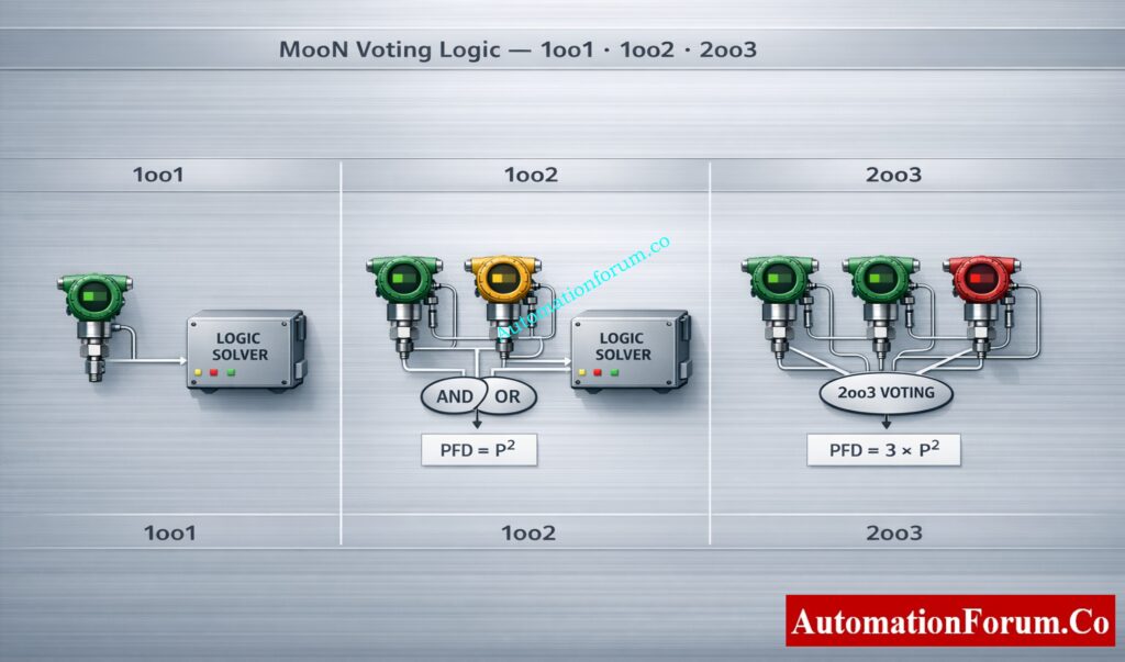

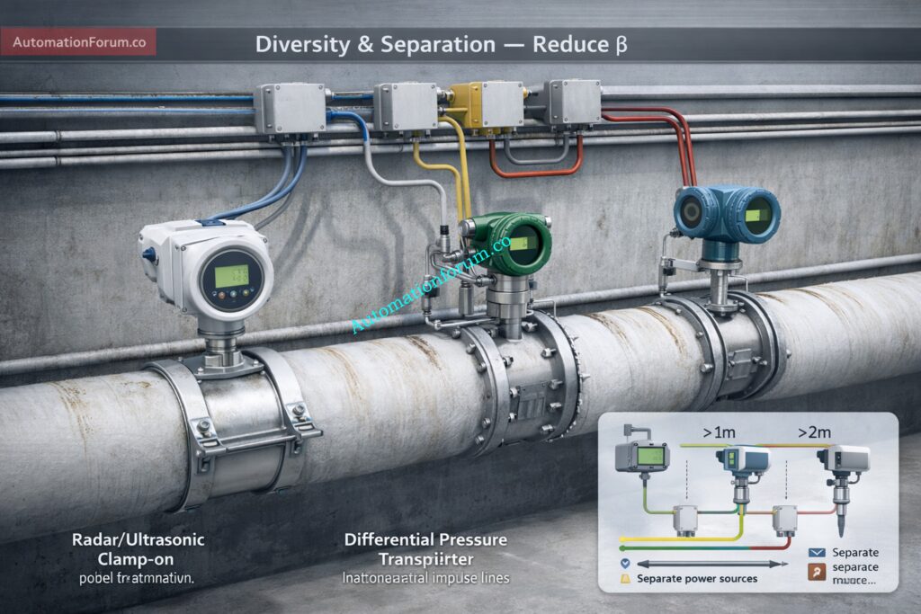
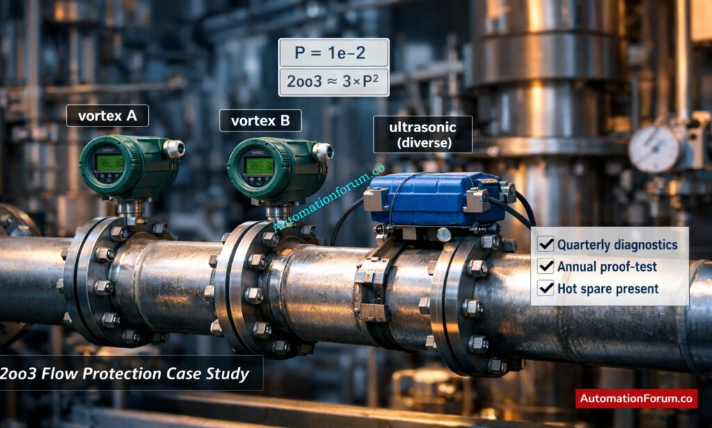
 Practical Guide for EPC Instrumentation & Process Automation Engineers 1")