PID controller tuning

Terminology

• PB – Proportional band.
• I.A.T. – Integral action time.
• D.A.T. – Derivative action time.
• M.V. – Measured value.
• P.V. – Process value.
• S.P. – Setpoint.
• C.V. – Control valve
• Po – Period oscillation time.
• P.B.µ – Ultimate proportional band. 
• Pµ – Ultimate period. 
• Pµ – Calculated time duration of one complete constant oscillation.
• PBc – Calculated Proportional band.
• ΔP% = Change in output to control value in %.
• Td = Apparent dead time in min.
• Tc = Apparent time constant in mins.
• ΔM.V.% = change in measured value in %.

What is the purpose of controller tuning?

Tuning of control system

• A control system on a process plant should be able to cope with load or setpoint (SP) changes with the minimum of disturbance to the process. 
• The purpose of tuning a controller is to determine the optimum controller parameters, i.e Proportional band(PB), Integral action time (I.A.T) and Derivative action time (D.A.T), so that this is achieved.

The response produced by the process to a load or S.P change after the optimum controller parameters have been set, is known as the “optimum response”. The optimum response differs from process to process. However, the most common criteria is to adjust the controller parameters so that the measured value(M.V) or process value(PV) response to a load or S.P change has an amplitude ratio or decay of 1:4, i.e the ratio of the overshoot of the second peak compared to the first is 1 to 4 as shown below.

What is quarter decay ratio response?

¼ Decay Optimum response

The M.V response shown is for a process that has been subjected to a load change.

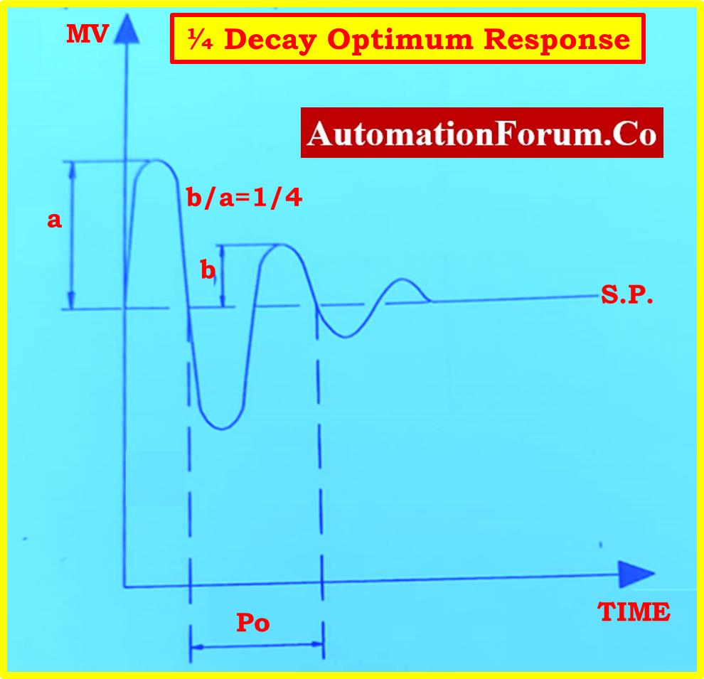
The response is a compromise between a rapid initial response and a short setting time. The period oscillation Po is the time taken for one cycle to occur.

What are the different PID tuning methods?

Techniques for Tuning Controllers

Techniques used for tuning controllers fall into two classes:-

1. Closed loop methods
2. Open loop methods

What is closed-loop PID tuning?

Closed Loop Methods

In these methods of controller tuning the controller parameters are based upon values determined from the closed loop response of the system, ie. with the controller on automatic.

The closed loop response methods which we will examine are:

• Ultimate sensitivity method
• Damped oscillation method

What is Ziegler-Nichols ultimate gain method?

Ultimate Sensitivity Method

Ziegler and Nichols of the Taylor Instrument Company came up with this technology in 1942, making it one of the first ways of tuning controllers was established.

The term “ultimate” was attached to this method because it requires the determination of the ultimate proportional band (or gain) and the ultimate period. 

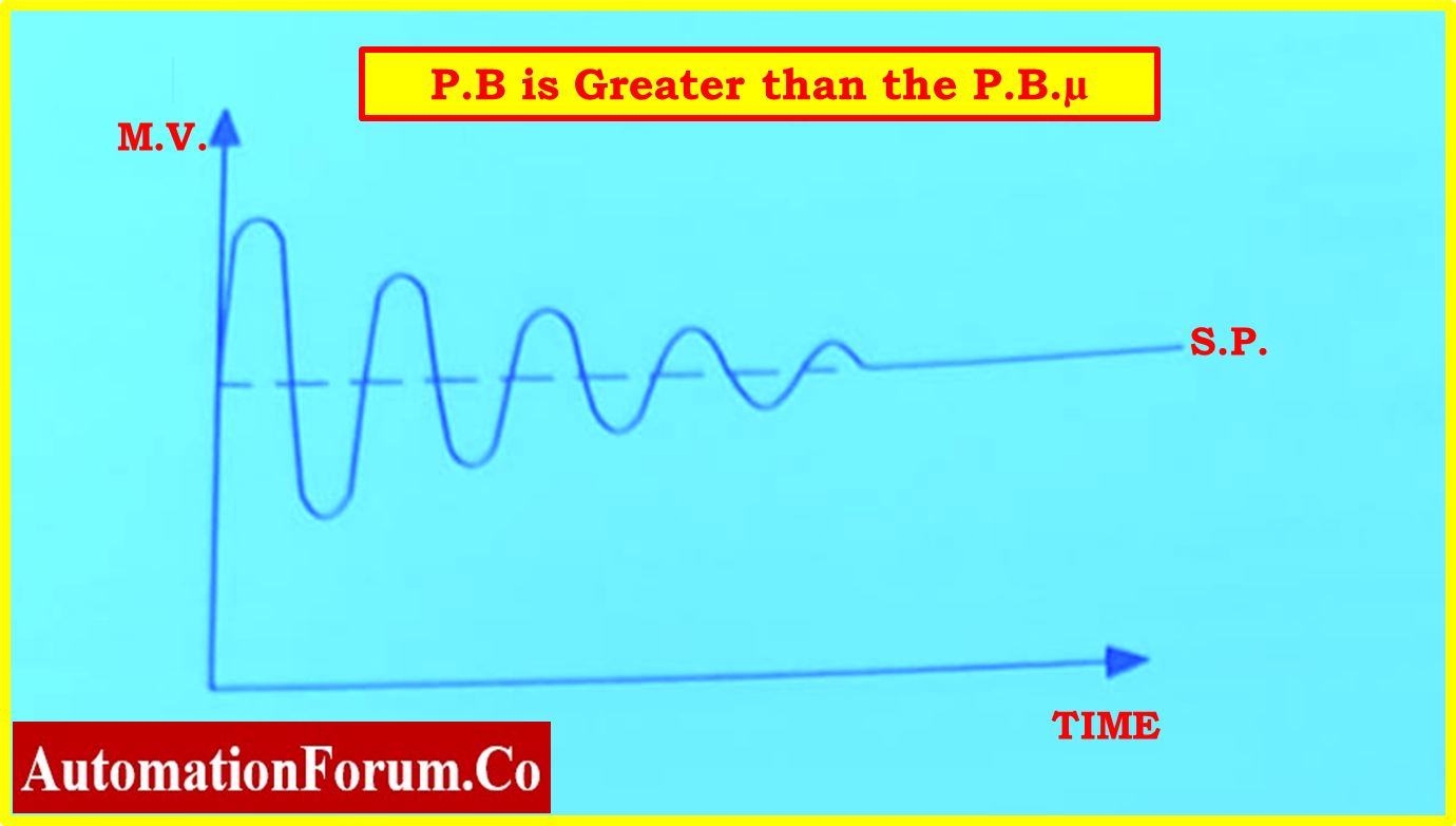
The ultimate proportional band P.B.µ is the minimum allowable value of P.B (for a controller in the proportional mode) for which, the system is stable, The ultimate period Pµ is the time taken for one cycle with the P.B at its ultimate value.

 The below diagrams show the M.V response to a step change when’-

The P.B is Greater than the P.B.µ

The P.B is less than the P.B.µ

The P.B = P.B.µ

Having found the ultimate PB and ultimate period then other controller parameters can be calculated using these values.

A full procedure for tuning control loops using this method is given below.

A fast speed chart recorder or storage oscilloscope is required to measure the M.V response to S.P/load changes.

Procedure

1. With the controller in manual adjust the P.B to a safe initial value (if unsure what a safe value is set P.B to its highest value).

set the other control parameters to their least effective value, i.e I.A.T to its maximum time and D.A.T to its minimum time.

2. Ensure M.V = S.P. switch controller to auto and allow system to stabilize.
3. Simulate a load change by making a small S.P change either up or downscale (a S.P change of a few % should be enough).
4. Observe the M.V response to the S.P change. If the M.V does not move towards the S.P and oscillate with small but constant amplitude, as shown previously, then the P.B will need to be adjusted.
5. Switch controller to manual.
6. The response obtained in step no.4 is initially more than likely to be sluggish. Therefore reduce the P.B setting (ensure you do not reduce the P.B too much as to narrow a P.B will result in the loop becoming unstable when put into auto).

If the response obtained in step no. 4 is unstable then the P.B will need to be increase. There is no definitive value to increase or decrease the P.B by. If in doubt then only make small adjustments until you have a better feel for the system.

7. Having adjusted the P.B repeat steps 2 to 6 until the ultimate P.B has been found.
8. Having found the ultimate P.B switch controller to manual

The controller parameters can now be calculated as shown below:-

Controller with Proportional Only:-

P.B = 2 XP.Bµ

Controller with Proportional + Integral:- 

P.B = 2.2 x P.Bµ

I.A.T = 0.8 x Pµ

Controller with Proportional + Integral + Derivative:-

P.B = 1,6 XP.Bµ

LA.T = 0.5 x Pµ

D.A.T = Pµ ÷ 6 = 5 secs = 5 ÷ 60 = 0.083

9. Set controller parameters to values calculated above.

10. Ensure M.V = S.P and switch controller to auto.

11. The controller should now be tuned correctly. Check this by making a small S.P. change and observing the M.V response.

12. The M.V response should be a 1/4 decay. If it’s not, you should examine your calculations.

13. If your calculations are correct then the controller may need fine tuning (remember put the controller on manual before adjusting any controller parameter).

From results if found the Gain = 5 then the PB would = 20% and the time Pµ = 30 secs we can put these figures into the formula to calculation the settings. PBc = calculated PB

e.g PBc = 1.6 x 20= 32% = a Gain of 3.125

IAT = 0.5 x 30 = 15 secs = 4 Repeats Per Min or a RR 0,25 mins per repeat

DAT = 30 ÷ 6 = 5 secs = 5 ÷ 60 = 0.083 DAT setting

From controller manual calculation settings for RR by using the time in minutes or % of. 30secs = 0.5

Reset R = 1.5 ÷ 0.5= IAT of 3 RPM or RR 0.33 mins per repeat

Preact = 0.5 ÷ 6 = 0.083

Then in auto adjust the PB in small increments to give the optimum control with these settings

What is damped oscillation method?

Damped Oscillation Method

This method is often called the 1/4 decay method of tuning. It was again developed by Ziegler & Nichols. The controller parameters are adjusted until a ¼  % decay response of the M.V is  obtained following a load change / S.P change. A fast speed chart recorder or storage oscilloscope is used to measure the response of the M.V to the S.P load change. 

Procedure

1. With the controller in manual adjust the P.B to a safe initial value (if unsure what a safe value is set P.B to its highest value). Set the other control parameters to their least effective value, i.e I.AT to its maximum  time and D.A.T to its minimum time.

2. Ensure M.V = S.P. switch controller to auto and allow system to stabilize.

3. Simulate a load change by making a small S.P change either up or downscale (a S.P. change of a few % should be enough).

4. Observe the M.V response to the S.P change. If the M.V response is not a 1/4 decay then the P.B will need to be adjusted.

5. Switch the controller to manual.

6. The response obtained in step 4 is initially more than likely to be sluggish. Therefore reduce the P.B setting (ensure you do not reduce the P.B too much as to narrow a P.B will result in the loop becoming unstable when put into auto). 

If the response obtained in step 4 is unstable then the P.B will need to be increase.

Note: There is no definitive value to increase or decrease the P.B by. If in doubt then only make small adjustments until you have a better feel for the system.

7. Having adjusted the P.B repeat steps 2 to 6 until a 1/4 decay response of the M.V following a S.P change is obtained.

8. If the controller is a P only type then the loop is now tuned correctly.

9. If the controller is a P+I or P+I+D type then measure the period of oscillation Po in minutes.

10. Switch controller to manual.

The control parameters can now be calculated using the information below:-

Proportional + Integral Controller:-

PBC = P.B / 0.9

LA.T = Po

Proportional + Integral + Derivative Controller:-

PBc = P.B / 1.2

I.A.T = Po x 0.6

D.A.T = Po / 6 = X secs thus X / 60 = DAT setting for the controller

11. Set controller parameters to values calculated above.

12. Ensure M.V = S.P and switch controller to auto.

13. The controller should now be tuned correctly. Check this by making a small S.P change and observing the M.V response.

The M.V. should have a 1/4 decay. If it’s not, you should examine your calculations.

If your calculations are correct then the controller may need fine tuning remember to put the controller on manual before adjusting any controller parameter).

What is open-loop method of tuning?

Open Loop Methods

In these methods of controller tuning the controller parameters are based on values determined from the open loop response of the system, i.e with the controller in manual. We will consider one particular method which is the “Process Reaction Curve method”.

What is meant by process reaction curve method of PID controller tuning?

Process Reaction Curve Method

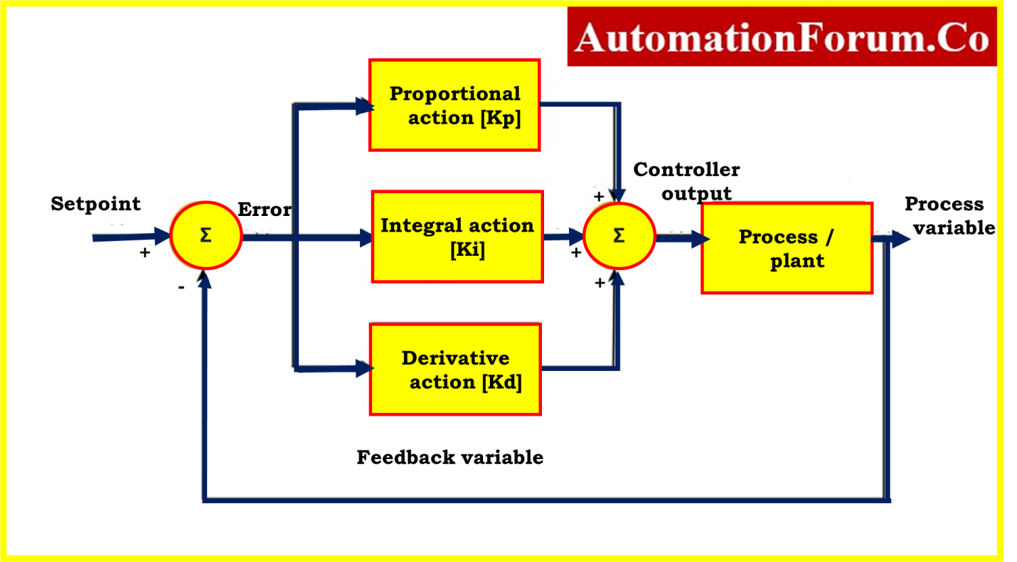
Again this method was originally developed by Ziegler & Nichols. Consider the block diagram shown below:-

It can be seen that the controller is set to manual control. A step change is then made using the manual output adjustment of the controller and the resulting process response is observed. The name for this kind of response is the “process reaction curve.”

Typical Response of the controller

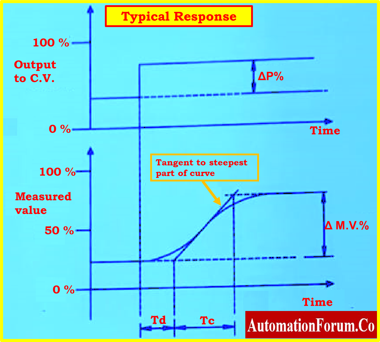
ΔP% = Change in output to control value in %.

Td = Apparent dead time in min.

Tc = Apparent time constant in mins.

ΔM.V.% = change in measured value in %.

Using the information obtained from the process reaction curve the controller parameter now be calculated using the following information-

Proportional Only Controller:

P.B ={ 100 x (ΔM.V ÷ Tc ) x Td} ÷ ΔP

Proportional + Integral Controller:

P.B ={ 110 x (ΔM.V ÷ Tc ) x Td} ÷ ΔP

IAT = 3.33 x Td

Proportional + Integral + Derivative Controller

P.B ={ 83 x (ΔM.V ÷ Tc ) x Td} ÷ ΔP

IAT =2x Td

DAT = 0.5 x Td

When using this method on a live system the following procedure should be followed

Procedure

1. Ensure M.V is at a suitable value and put controller into manual (make a note of M.V at this stage).
2. Allow the process time to stabile and the make a step change of the controller output
3. Be careful to record a “process reaction curve” in the appropriate format.
4. Return controller output to its previous value and ensure M.V returns to value noted in step 1.
5. Calculate the controller using the “process reaction curve” and information given previously.
6. Set the controller parameters to values calculated.
7. Ensure M.V – S.P and switch controller to auto.
8. The controller should now be tuned correctly. This can be checked by making a SP change and observing the M.V response.

The M.V. should have a 1/4 decay. If it’s not, you should examine your calculations.

If your calculations are correct then the controller may need fine tuning remember to put the controller on manual before adjusting any controller parameter).

What is trial and error tuning method?

1. The trial-and-error method is also known as the manual tuning method, and it is the simplest method.

2. Increasing the value of Kp until the system achieves an oscillating response is the first step in this method.

3. However, the system should not become unstable, and the values of Kd and Ki should remain unchanged.

4. After that, adjust the value of Ki such that the oscillation of the system is brought to an end. After then, adjust the value of Kd such that it provides a quick reaction.