Quiz Scope: Transmitter Faults, Signal Issues and Installation Pitfalls
This quiz is for process, instrumentation, and maintenance engineers who are already good at fixing vortex flow meters. It includes problems with transmitters, signal conditioning and wiring, HART/4-20 mA problems, the effects of noise and vibration, flow profile and piping effects, the effects of temperature and pressure, zero/span drift, calibration and loop-check procedures, firmware/configuration problems, and safety-related diagnostics. Expect scenario-based questions that ask you to find the core cause of a problem, isolate the defect step by step, and take practical steps to fix it. Field recommendations show you how to take good measurements and do tests. Use this to assess skills, improve commissioning checks, and make plant uptime plans stronger for both custody transfer and process control applications. Answers make it apparent what diagnostics, remedial actions, and preventive maintenance measures are.
Quick Start: Why Vortex Flow Meter Troubleshooting Matters
Forward Acting Control Valve vs Reverse Acting Control Valve: Selection Guide
Control valves are the backbone of any process control system. In industries such as oil and gas, petrochemical, power generation, and manufacturing, they act as the final control element that directly influences process variables like flow, pressure, temperature, and level.
When designing a plant in real life, engineers generally spend a lot of time choosing transmitters, setting up controllers, and adjusting PID loops. However, one of the most critical and frequently misunderstood decisions is selecting the correct control valve action.
From field experience, incorrect selection between a forward acting control valve and a reverse acting control valve can result in:
Unstable control loops
Opposite process response
Poor controllability during disturbances
Dangerous plant conditions during failure scenarios
In EPC projects, it is common to see loop performance issues traced back not to controller tuning, but to incorrect valve action or fail safe configuration. A poorly selected valve can make even a well tuned control loop behave unpredictably.
Understanding valve action is therefore not just a theoretical requirement. It is a practical necessity for safe and stable plant operation.
When to Use Forward Acting Control Valve in Process Industries
Forward Acting Control Valve in Cooling Water Systems
A forward acting control valve is selected when an increase in the control signal must result in an increase in flow or process effect. In simple terms, the valve movement follows the direction of the signal, meaning signal up leads to valve opening up. This direct relationship between controller output and valve position is fundamental in many process applications where increasing the manipulated variable helps correct the process deviation.
From an instrumentation design engineering perspective, forward acting valves are preferred in systems where the process requires immediate reinforcement of flow or removal of energy as the process variable increases.
Cooling System Control Logic Temperature Increase Flow Increase
In cooling applications, the process variable is typically temperature, and the objective is to remove heat efficiently.
Increase in temperature requires more cooling
Controller detects high temperature and increases output
Valve must open to allow more cooling medium
Why Fail Open Valve is Preferred in Cooling Applications
This makes forward acting control valves highly suitable for cooling water circuits, heat exchangers, and jacket cooling systems.
In practical plant design:
Reactor temperature rises
Controller output increases
Cooling water valve opens further
This ensures that heat removal increases proportionally with temperature rise.
From field experience, incorrect valve action in cooling loops often results in dangerous scenarios. If the valve closes when temperature rises, the system will move toward thermal runaway instead of stabilizing.
Pressure Increase Vent Valve Opening Strategy
In pressure control situations where venting or relief is needed:
More discharge or venting is needed when the pressure goes up.
As pressure goes up, the controller output goes up.
To alleviate too much pressure, the valve must open.
Forward Acting Valve in Flare and Vent Gas Systems
Forward-acting valves make sure that pressure is lowered promptly and effectively.
Typical applications include:
Flare systems
Vent gas systems
Compressor anti surge lines
To stop pressure from building up in these systems, there must be a direct link between the signal and the valve opening.
Forward Acting Control Valve in Flow Control Applications
In standard flow control applications:
Increase in controller output should increase flow
Valve opening must increase proportionally
Flow Loop Design Using Direct Acting Valve
This is the most straightforward application of forward acting control valves and is widely used in:
Feed flow control
Transfer lines
Utility distribution systems
Since the process gain is positive in these cases, a direct relationship between signal and flow is required for stable control.
Refer the below link for the Understand Essential Control Valve Performance Parameters
When to Use Reverse Acting Control Valve in Process Industries
When a control signal has to go up, a reverse acting control valve is used to make the flow or process effect go down. In this example, the valve moves in the opposite direction of the signal, thus when the signal goes up, the valve closes.
Most of the time, these valves are utilized in systems where adding energy or material is part of the process, and lowering the input is needed to raise the process variable.
Reverse Acting Control Valve in Heating Systems
In heating applications, the goal of the process is to keep the temperature stable by managing the amount of energy that goes in.
If the temperature goes up, the heating needs to go down.
This checklist helps avoid common design, commissioning, and operational errors while ensuring that the selected valve action supports both process stability and plant safety.
Choosing between a forward acting control valve and a reverse acting control valve is a fundamental decision in instrumentation design engineering.
It directly affects:
Process safety
Loop stability
Plant reliability
From field experience, the best engineers do not rely on memorized rules. They analyze:
Process behavior
Energy addition or removal
Failure scenarios
A properly chosen valve makes sure that:
Control loops that stay the same
Response to the procedure that can be predicted
Safe operation under unusual situations
In the end, it’s more crucial to understand the process than to choose the valve. The valve action must always follow the process logic, not the other way around.
Select the right control valve based on process gain, fail safe requirement, and whether the system needs heating or cooling. Always evaluate what happens during air failure and ensure valve action matches process control logic.
What is the difference between PCV and LCV?
A PCV controls and maintains system pressure, while an LCV controls liquid level in tanks or vessels. The difference is based on the process variable being controlled pressure versus level.
What is the rule of thumb for control valve sizing?
A common rule is to size the control valve so it operates around 60 to 80 percent opening at normal conditions. This ensures good controllability, avoids cavitation, and allows margin for process variation.
The purpose of reverse acting control is to reduce process input when the process variable increases. It helps maintain stability in systems where increasing output must decrease flow or energy.
What is Zener vs Galvanic Isolation in Intrinsic Safety Loops
Intrinsic safety loops using 4 to 20 mA signals are widely used to keep instrumentation circuits safe in hazardous atmospheres. The choice between a Zener barrier and a galvanic isolator affects grounding practice, available loop voltage, diagnostics, maintenance and long term reliability. This article provides practical selection rules, detailed wiring and installation notes, conservative numerical examples and commissioning checks for instrumentation and control engineers in EPC and operations teams.
What is a Zener Barrier in Intrinsic Safety Systems
A Zener barrier is an energy limiting device installed in the safe area to prevent energy levels that could ignite a flammable atmosphere from reaching field devices in the hazardous area. The barrier limits both voltage and current using a combination of passive components and a sacrificial fuse.
a series resistor sized to limit current under fault conditions,
one or more Zener diodes that clamp voltage to a defined maximum,
a fuse that opens the feed if a sustained overcurrent occurs,
a dedicated protective earth connection used to divert clamped energy to ground.
Under normal operation the series resistor and diode network allow the loop to operate and the transmitter to receive sufficient voltage and current. Under a fault such as a short or a power supply failure, the Zener diode clamps voltage and the resistor limits the current to safe levels. If the current remains high long enough, the fuse clears and isolates the circuit.
Zener Barrier Components Resistor Zener Diode Fuse and Earth
There are two practical barrier categories encountered in the field. The first is the low cost passive Zener barrier commonly used on single loop installations. The second is an active barrier where additional electronics reduce voltage drop and provide better defined available voltage to the field device while retaining the Zener clamp and fuse protection. Selection depends on required loop headroom, whether diagnostics and HART communication are required, and the plant earthing policy.
Zener Barrier Grounding Requirements and IS Loop Earthing Rules
The protective earth connection is mandatory for the barrier to perform correctly. If the earth connection is missing, loose, or takes a long path back to plant earth, the barrier may not divert dangerous energy properly. For that reason plant design must specify earth conductor sizing and routing and inspection during commissioning.
Advantages and Limitations of Zener Barriers in Process Plants
Simple and cost-effective solution for intrinsic safety in basic 4 to 20 mA loops with easy installation and maintenance.
Requires a reliable low-impedance earth and reduces available loop voltage, which can limit cable length and loop performance.
Best suited for simple, short-distance applications but less flexible for complex systems, HART communication, and multi-loop setups.
What is a Galvanic Isolator in Intrinsic Safety Applications
A galvanic isolator provides full electrical separation between the safe area circuit and the hazardous area circuit. Isolation is achieved by means of an isolating transformer, optocoupler or active electronic isolation stage. Isolators are available as loop powered two wire devices and as three port devices that separate input, output and supply.
Refer the below link for the What is SIS, SIF and SIL? An In-Depth Guide to Functional Safety in Process Industries
How Galvanic Isolation Works Using Transformer Optocoupler and Electronics
Common implementations are:
transformer based isolator where magnetic coupling transfers the signal while blocking dc continuity,
optocoupler based isolator where light transmits the signal across an insulating barrier,
active electronic isolator where dedicated circuitry and dc to dc conversion provide isolation and regulated outputs.
Types of Galvanic Isolators Loop Powered and Three Port Isolators
A three port isolator separates the hazardous area loop, the safe area loop and the supply. That architecture allows a safe area earth free installation of the hazardous area side and removes the need to create a dedicated protective earth for safety reasons.
Benefits of Galvanic Isolators for Industrial Instrumentation Systems
Galvanic isolation offers these practical benefits:
does not require a safety earth on the hazardous area side to perform the energy separation function,
provides higher available loop volts so long cable runs or higher loop resistance are supported,
reduces the risk of ground potential differences causing noise or damaging signals,
often includes built in repeat, conversion or HART passthrough capability which aids diagnostics and integration.
Limitations and Design Considerations of Galvanic Isolators
Isolators are active devices and can be more expensive per channel than a simple Zener barrier. They may require local power or specified loop powering arrangements. For safety certification they must be certified for the intrinsic safety concept in use and installed per manufacturer instructions.
Proper Earthing and Grounding Practices for Zener Barriers
Connect a separate protected earth conductor from the Zener barrier earth terminal to the plant’s protective earth system. Copper should be used for the earth conductor, and it should be the right size and installed according to plant electrical regulations.
Make the road to the ground as short and direct as you can. Don’t run the earth wire through panels, structures, or conduits that can create extra impedance and make it less effective.
Check the earth continuity and make sure the resistance matches the plant’s needs, which is usually less than 1 ohm, during installation and commissioning. Write down the numbers for earth impedance and put them in the commissioning paperwork so you can look them up later.
To avoid differences and dangerous situations, make sure that all barriers have the same reference ground point.
Cable Routing Shielding and Noise Reduction Techniques
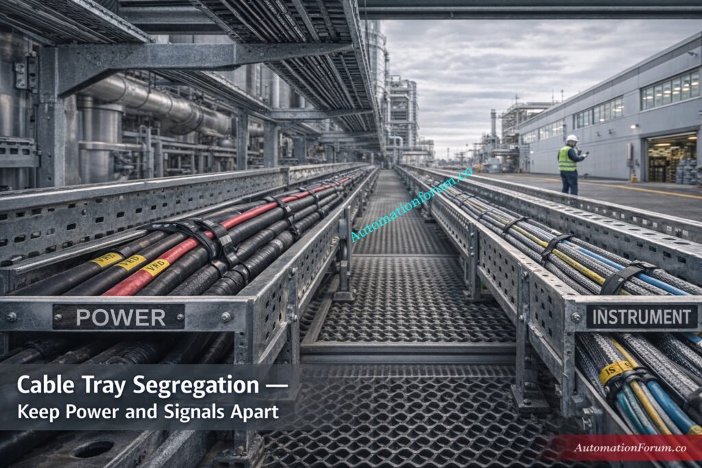
To stop electromagnetic interference and signal distortion, keep inherent safety cables away from power cables, high voltage lines, and switching circuits.
Hazardous area wiring guidelines say that cable trays and conduits should have enough space between them. Don’t run high-current wires in parallel across extended distances.
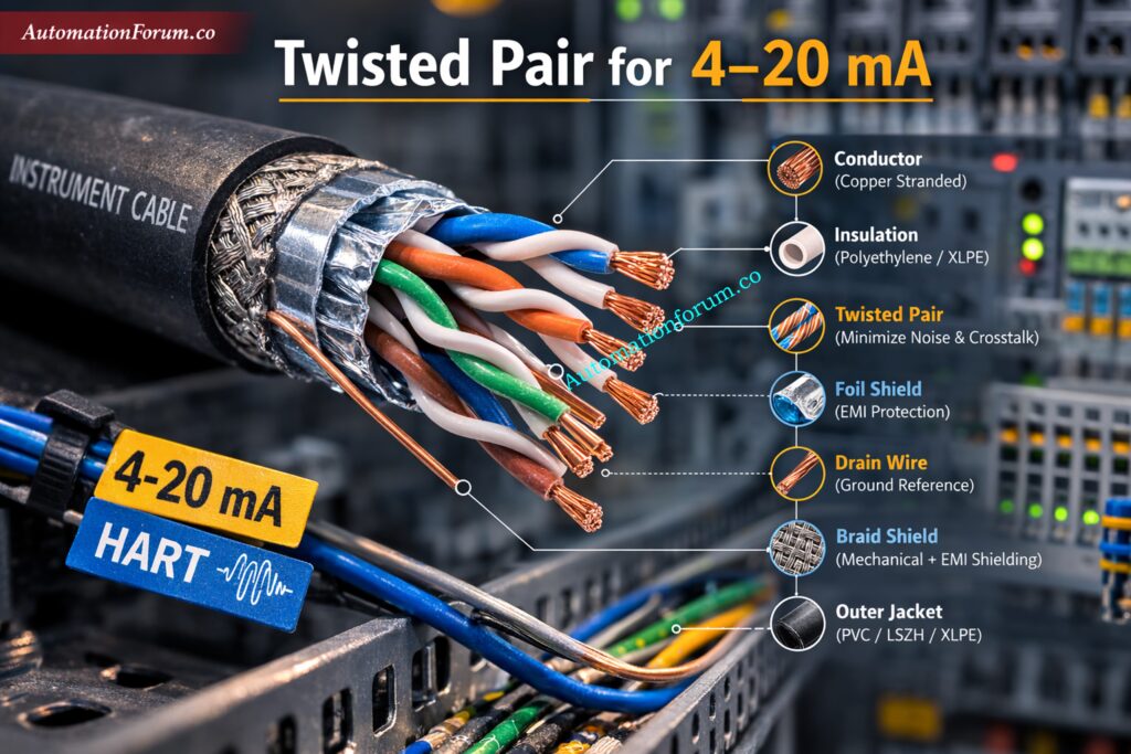
For sending analog signals over lengthy cable runs, use insulated twisted pair cables. This makes the signal more accurate and less likely to pick up noise.
Only connect cable shielding at the safe area end, unless the plant’s grounding philosophy says otherwise. Bad shielding can cause ground loops and noise problems.
Make sure that the documentation for cable identification and routing is correct so that troubleshooting and maintenance can be done.
Installation Best Practices for IS Loops in Hazardous Areas
Put Zener barriers and galvanic isolators in safe area enclosures like control room cabinets or marshalling panels so they are easy to get to and safe.
Make sure that the wiring for intrinsic safety and non-intrinsic safety is kept separate inside the panels. Use partitions or separate wiring ducts to keep things separate.
Make sure to clearly mark all of the loop numbers, barrier terminals, earth connections, and fuse ratings. This makes maintenance easier and troubleshooting faster.
Follow the manufacturer’s installation instructions exactly, including the polarity of the wire, the torque on the terminals, and the circumstances in the environment.
Keep your loop diagrams and wiring drawings up to date so that they show how things are actually set up for operational clarity.
Common Installation Mistakes and How to Avoid Them
Do not connect Zener barrier earth terminals to local pipework, cable trays, or floating metal structures unless you are sure they are part of the plant’s protective earth system.
Don’t make more than one earth path for the same barrier system. This can cause currents to flow in a circle, noise problems, and lower intrinsic safety performance.
Make sure that barrier fuses are not bypassed or replaced with ones that have the wrong ratings. To keep your safety certification, always use the fuse kinds that the manufacturer says to.
You shouldn’t mix intrinsic safety and non-intrinsic safety wiring without sufficient separation, as this could break hazardous area requirements.
Check installations often for loose connections, broken wires, or wrong routing to avoid problems with reliability in the long run.
Loop Resistance and Voltage Drop Calculation Example
This example shows how Zener barriers and galvanic isolators affect loop resistance and available voltage in 4 to 20 mA intrinsic safety loops.
Zener Barrier Loop Loading Calculation with Example
Assume a 24 volt supply and a two wire transmitter operating at 20 mA.
Available voltage from the Zener barrier is approximately 16.0 volts at full load.
Maximum loop resistance Rmax = 16.0 divided by 0.02 = 800 ohms, but use a practical design limit of 600 ohms to allow margin.
Galvanic Isolator Loop Loading Calculation with Example
With a typical isolator voltage drop of 3 volts, about 21 volts is available to the transmitter.
Maximum loop resistance Rmax = 21 divided by 0.02 = 1050 ohms.
Use a conservative design limit of around 900 ohms for reliable operation and HART communication.
Practical Design Limits for Long Cable Runs
Use Zener barriers for short loops with low resistance and stable grounding conditions. Select galvanic isolators when loop resistance exceeds 600 ohms or cable runs are long.
Always verify calculations using manufacturer data to ensure sufficient voltage margin and loop stability.
Real Industrial Case Studies Zener vs Galvanic Isolation
Case Study Zener Barrier for Short Distance Flame Detector Loop
A flame detector in a dusty zone is located five meters from the junction box. The instrument is two wire and requires basic HART diagnostics only occasionally. Plant earth at the control room is robust and short earth conductors can be run to the barrier location. A passive Zener barrier is selected due to low capital cost and ease of local maintenance. The installation includes labeled spare fuses in the local instrument cabinet and a simple commissioning test sheet that includes earth continuity fuse checks and loop resistance measurement. The design limits loop resistance to 500 ohms to preserve HART margin.
Case Study Galvanic Isolator for Remote Transmitter System
A remote transmitter rack sits on a floating platform with no reliable protective earth and cable runs to the control room exceed 800 meters. Multiple 4 to 20 mA loops require HART diagnostics and occasional rerouting. A three port galvanic isolator rack is specified to provide isolation between the hazardous area loops and the safe area I O shelf while allowing HART to pass. The isolator reduces risk from earth loops and gives sufficient loop headroom for long cable resistance. The solution requires higher initial cost but lower maintenance overhead and reduced risk of nuisance tripping or incorrect earthing.
Frequently Asked Questions Zener vs Galvanic Isolation
What is the difference between Zener barrier and galvanic isolators?
A Zener barrier limits voltage and current using diodes and requires a dedicated earth. A galvanic isolator provides complete electrical isolation without needing an IS ground.
What is the purpose of a galvanic isolator?
It isolates hazardous and safe area circuits to prevent fault energy transfer. It also improves signal integrity and eliminates ground loop issues.
What is the difference between galvanic isolation and optical isolation?
Galvanic isolation blocks electrical continuity using transformers or capacitive methods. Optical isolation is a type of galvanic isolation that uses light via optocouplers.
Are galvanic isolators intrinsically safe?
Yes, when certified, they are used as associated apparatus in IS systems. They limit energy transfer while maintaining isolation between circuits.
How to check galvanic isolation?
Use an insulation tester to verify high resistance between input and output circuits. Confirm no direct electrical continuity and check isolation voltage ratings.
What is the purpose of a Zener barrier?
It limits voltage and current entering hazardous areas to prevent ignition. It safely diverts excess energy to earth using Zener diodes and resistors.
Can I mix Zener barriers and galvanic isolators in one installation?
Yes mixing is common. Keep wiring diagrams explicit and ensure each loop follows the installation practices required by the device used.
What is the most common cause of Zener barrier failure in service?
A blown fuse or a poor earth connection are the most common issues. Both are visible faults if regularly inspected.
Will a galvanic isolator always allow HART communication?
Not always verify HART passthrough explicitly in the product data and perform a HART test during commissioning.
Does a galvanic isolator remove the need for careful cable routing?
It reduces sensitivity to earth loops but standard cable segregation shielding and routing practice still applies.
How often should barrier fuses be inspected?
Inspect visually during routine maintenance and test as part of periodic loop verification. Replace only with manufacturer specified fuse types.
Why is galvanic isolation preferred in modern plants?
It eliminates dependence on dedicated IS grounding and avoids ground loop noise issues. It also supports longer cable runs with improved signal stability and accuracy.
Does a Zener barrier affect loop resistance?
Yes, it reduces available loop voltage, limiting maximum allowable resistance. This can restrict cable length and impact transmitter performance.
Do galvanic isolators support HART communication?
Most modern isolators allow HART signal passthrough without distortion. Always confirm HART compatibility in the manufacturer datasheet.
Is grounding required for galvanic isolators?
No dedicated IS earth is required for intrinsic safety operation. However, proper system grounding practices must still be maintained.
What happens if a Zener barrier fuse blows?
The loop becomes open circuit and the field device stops operating. The fuse must be replaced with the exact specified rating before restoring service.
Refer the below link for the Why Choose Intrinsic Safety (IS) for Hazardous Area Instrumentation?
Your Trusted Source for Automation Power Tools & Solutions
IEEE 80IEEE 142 · Green BookIEC 60364ISA RP12.6PLC GroundingDCS EarthingSignal Ground4–20 mA Loop
PSU
CPU
DI
DO
AI
AO
COM
PLC / CONTROL PANEL STATUS
RUNCOMM OKHARTPROFIBUS4–20 mAMODBUS
Input Parameters
Results
Single Rod
—Ω
Dwight formula
Total Ground
—Ω
R / √n parallel
Reduction
—%
vs single rod
Formula Reference
R = (ρ / 2πL) × ln(4L / d)
R_total = R / √n
ρ Soil resistivity (Ω·m) ·
L Rod length (m) ·
d Rod diameter (m) ·
n Number of rods
Reference & Standards
Grounding Targets
< 1 Ω — Excellent
1–2 Ω — Acceptable
2–5 Ω — Needs improvement
> 5 Ω — Poor / remediate
Standards Applied
IEEE 80 — Substation grounding
IEEE 142 — Green Book
IEC 60364 — LV installations
ISA RP12.6 — Instrument ground
PLC / Instrument
PLC chassis — < 1 Ω
DCS cabinets — < 1 Ω
Signal ground — < 5 Ω
HART / 4-20 mA — < 2 Ω
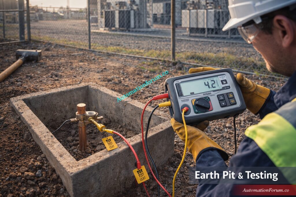
Instrument Earthing and Industrial Grounding Systems
Proper instrument earthing is one of the most important foundations of a reliable industrial automation system. In process industries such as oil and gas, petrochemical plants, refineries, power plants, and water treatment facilities, thousands of instruments and control systems depend on stable electrical grounding to function accurately and safely.
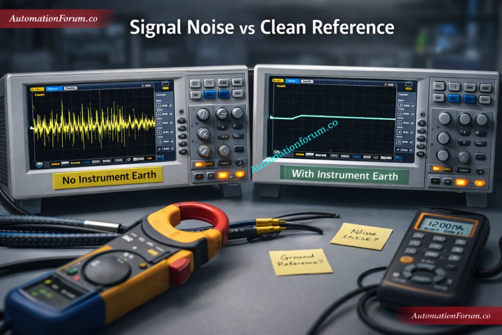
When the earthing system is poorly designed or has high resistance, several operational problems can occur. Engineers frequently encounter PLC communication failures, unstable 4 to 20 mA signals, instrument drift, erratic alarms in control systems, and potential damage to delicate equipment during lightning strikes or electrical surges. Not only are these problems hard to fix, but they can also cause expensive production delays.
Correct industrial grounding makes sure that electrical noise is securely sent to the ground and gives instrumentation signals a solid reference point. This is particularly critical for PLC grounding systems, distributed control systems, analyzers, and field instruments.
An Instrument Earthing Resistance Calculator is a practical engineering tool that helps engineers estimate the resistance of grounding electrodes before installation. By performing a quick earthing resistance calculation using soil properties and ground rod parameters, engineers can design an effective industrial earthing system that meets process plant grounding requirements and improves overall automation reliability.
Importance of Instrument Grounding in Industrial Automation Systems
Instrument earthing refers to the practice of connecting instrumentation equipment and control systems to a stable earth reference to ensure safety, signal stability, and protection against electrical disturbances.
In process plants, instrumentation systems include pressure transmitters, temperature transmitters, flow meters, PLC systems, distributed control systems, analyzers, and field junction boxes. These devices rely on accurate electrical signals to measure and control industrial processes. Any disturbance in the grounding system can affect signal accuracy and system reliability.
Types of Instrument Grounding Used in Process Plants
Instrumentation grounding is typically categorized into three types.
Protective Earthing for Electrical Safety
Protective earthing is designed to protect personnel and equipment from electrical faults. If an electrical fault occurs, the fault current flows through the earthing conductor to the ground, allowing protective devices such as circuit breakers to operate safely.
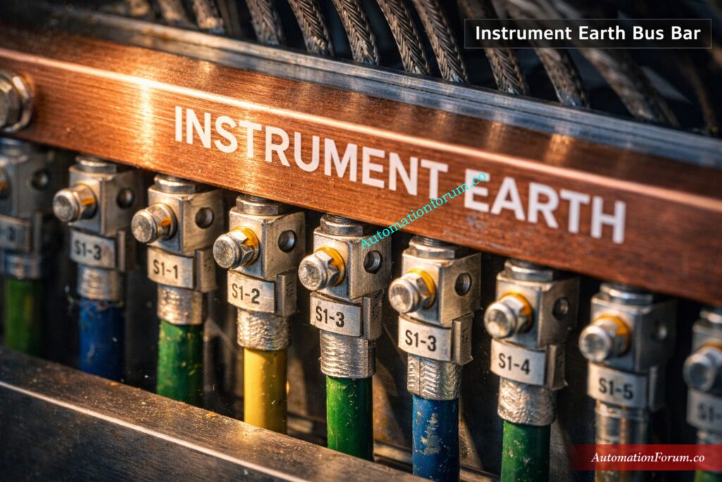
Signal Grounding
Signal grounding provides a stable reference for measurement signals. Analog signals such as 4 to 20 mA loops require a clean electrical reference to avoid noise interference and measurement errors.
Signal Grounding for 4 to 20 mA and Communication Signals
This type of grounding provides a common reference point for sensitive instrumentation equipment such as PLC cabinets, analyzer systems, and control system electronics.
In many industrial facilities, instrumentation grounding is kept separate from heavy power grounding systems. Power equipment such as motors and transformers generate electrical noise and fault currents that can disturb sensitive instrumentation signals.
Typical Grounding Resistance Targets for PLC and Instrumentation Systems
Typical industrial targets (practical guidance, not absolute rules):
PLC / CPU chassis: < 1 Ω where possible for best communication stability.
4-20 mA signal reference: < 2 Ω recommended for critical loops.
General signal ground: < 5 Ω acceptable in many plants; remediation recommended if higher.
These targets are used by engineers during design and commissioning to determine whether a simple driven rod is enough or a grid/chemical treatment is required.
Overview of the Instrument Earthing Resistance Calculator
What is an Instrument Earthing Resistance Calculator
The Instrument Earthing Resistance Calculator is an engineering tool used to estimate the resistance of grounding electrodes installed in soil. It helps engineers evaluate whether a grounding system design will achieve acceptable resistance levels before the installation of ground rods.
Purpose of Earthing Resistance Calculation in Industrial Grounding Design
The calculator is based on the same engineering ideas that go into figuring out the resistance of a ground rod. It uses the resistivity of the soil and the size of the electrodes to figure out how easily electricity may flow into the ground.
The resistance of a vertical ground rod is mostly affected by three things:
soil resistivity length of the rod diameter of the rod
Refer the below link for Understanding the Dead Zero Problem in Industrial Analog Signals
How Multiple Ground Rods Reduce Total Grounding Resistance
To lower total resistance, many industrial setups include several rods. When rods are joined, they work together and lower the total grounding resistance.
The calculator figures out this total resistance by looking at how many rods are in the grounding system. With this earthing resistance calculator, engineers can easily test out several grounding setups and choose the best one for industrial earthing systems.
Key Parameters Used in the Instrument Earthing Resistance Calculator
For reliable earthing design, it’s important to know what each parameter means and how it affects the field. The calculator takes a few input data, like soil resistivity (ρ), ground rod length (L), rod diameter (d), number of rods (n), and rod spacing, and turns them into an estimate of resistance. Below are the parameters explained with engineering context and industrial examples.
Soil Resistivity and Its Impact on Grounding System Performance
Units: Ω·m. Soil resistivity is the single most influential variable. Clayey, moisture-rich soils have low resistivity (e.g., 20 – 200 Ω·m), whereas dry sand, gravel or rock can exceed 1,000 – 2,000 Ω·m.
Field practice: measure using a Wenner or fall-of-potential test across representative locations (near control rooms, tank farms, and proposed electrode locations). Don’t assume textbook values for site-specific design. Soil resistivity varies with depth, season and proximity to drainage.
Example: a coastal refinery marsh layer may show 30–80 Ω·m, whereas rocky plateau sites may show 1,000 – 2,000 Ω·m – design choices differ radically between them.
Ground Rod Length and Its Effect on Earthing Resistance
Units: meters. Longer rods reduce resistance roughly inversely with length in the formula. Typical driven rods in process plants are 2.4 m (8 ft) or 3.0 m. Where space allows, deeper rods (or driven pipe electrodes) are preferred.
Field note: rock or high groundwater tables may limit achievable depth. When you can get deeper than 3 m, resistance falls significantly.
Ground Rod Diameter and Mechanical Strength Considerations
Units: meters (often entered as mm in UI). Standard driven rods are 16 mm to 25 mm in diameter (solid copper or copper clad steel). Diameter has a relatively minor effect versus length and resistivity, but thinner rods have slightly higher resistance and lower mechanical strength. Use thicker rods where mechanical durability and corrosion resistance matter.
Number of Ground Rods and Parallel Grounding Design Principles
Installing multiple rods in parallel reduces total resistance, but returns diminish as spacing and soil overlap become limiting. The calculator uses the √n approximation to estimate the benefit of parallel rods as a first-order guide.
Practical example: four rods in good soil may reduce resistance to roughly half a single rod – sufficient for many signal grounding applications; in high-resistivity sites you must either add many rods, increase depth, or install a ground grid.
Ground Rod Spacing and Avoiding Overlapping Resistance Zones
Proper spacing avoids overlapping ‘resistance zones’ around each rod. A common field rule-of-thumb is rod spacing ≥ 3·L (three times the rod length) to reduce interaction. If rods are too close, the √n approximation becomes optimistic.
Industrial practice: for three-meter rods, 9 m spacing is conservative; for 2.4 m rods, 7 – 8 m spacing. Where space is constrained, a ground ring or chemical treatment may be better than closely clustered rods.
Typical Grounding Parameter Values Used in Industrial Earthing Design
Soil resistivity: 30 – 2,000 Ω·m depending on site.
Rod length: 2.4 m (standard), 3 m (preferred).
Diameter: 16 mm copperclad (standard), 25 mm for mechanical robustness.
Number of rods: single for small cabinets; 2 – 6 for control rooms; many tens for substation-grade grids.
Spacing: 3 – 5 m minimum; 3·L is a conservative design approach.
Engineers must always pair calculator outputs with field measurements and local construction constraints. The calculator gives a first-order estimate to plan materials, layout and potential remediation.
It is effective in both the design stage (to choose rod size/quantity and preliminary layout) and the maintenance/commissioning stage (to interpret soil tests and decide remediation steps). Use it as a quick engineering estimator – not a substitute for a full substation grounding analysis when high fault currents are involved.
Essential Earthing Drawings Every Engineer Must Understand: Earthing Drawing
How to Use the Instrument Earthing Resistance Calculator Step by Step
Below is a practical field procedure to use the calculator and interpret the results. The steps assume the calculator UI accepts direct numerical inputs and returns single-rod resistance, combined resistance and a guidance status.
Step 1 Identify Soil Type and Measure Soil Resistivity
Perform a Wenner four-pin test in-situ at the proposed electrode location and record ρ (Ω·m). If you don’t have a measurement, use conservative estimates (clay 20-100 Ω·m, moist soil 100-300 Ω·m, sandy 300-1,000 Ω·m, rocky >1,000 Ω·m). Enter the measured or chosen ρ in the calculator.
Step 2 Enter Ground Rod Length in the Calculator
Input the driven rod length in metres. Choose the deepest practical driven depth (2.4 m is common; 3.0 m is preferred if achievable).
Step 3 Input Ground Rod Diameter
Enter diameter in mm (the calculator will convert to metres). Standard selection: 16 mm copperclad (0.016 m).
Step 4 Specify the Number of Ground Rods Installed
For a single cabinet choose n = 1; for a control room or field marshalling kiosk, start n = 2-4; for large substations you will design a grid.
Step 5 Enter Ground Rod Spacing Distance
Provide spacing (m). If spacing is ≥ 3·L, the √n approximation is more valid. If spacing is closer, treat the calculator result as optimistic.
Step 6 Run the Earthing Resistance Calculation
Click Calculate. The calculator returns:
R (single rod) using R = (ρ / (2πL))·ln(4L/d)
R_total using R_total ≈ R / √n
% reduction relative to single rod.
Step 7 Interpret the Calculated Ground Resistance Result
Compare R_total to project targets: PLC chassis < 1 Ω preferred, 4-20 mA loops < 2 Ω, general signal ground < 5 Ω. If R_total > target, decide remediation.
Interpretation: 36.7 Ω is far above instrumentation targets remedial actions (deeper rods, many more rods, chemical treatment or a ground grid) are required. This step-by-step example shows that in moderate-to-high resistivity soils, driven rods alone rarely achieve <1 to 2 Ω without additional measures.
Take a look at this example:
Soil resistivity = 150 ohm meter Rod length = 2.4 meters Rod diameter = 16 mm Number of rods = 3
If you use the ground rod resistance calculation formula, you may figure out that one rod’s resistance is about 63 ohms.
The total resistance may go down to about 36 ohms when three rods are inserted.
If the goal grounding resistance is less than 5 ohms, you will need more rods or better grounding methods.
When to Use an Instrument Earthing Resistance Calculator in Process Plants
Use the earthing resistance calculator in real life, like when you need to:
When designing a grounding system, you need to figure out how many rods and how long they should be to reach the signal-ground aim before you finish the civil work.
During plant commissioning, we compare the expected resistances to the observed resistances. If the measured resistance is worse than the predicted resistance, it means that there are problems with the construction or the soil conditions.
When fixing instrumentation noise, if you think that PLC communication faults or 4–20 mA jitter are caused by the earth, utilize the calculator to see if the local chassis earth needs to be reinforced.
During earthing audits or safety inspections: to document expected resistance under different soil conditions and propose remediations.
During expansion of control systems: when adding remote I/O racks or analyzer shelters, quickly verify whether the existing earth will support additional loads.
The tool is best used in tandem with field measurements (Wenner tests or fall-of-potential data) and engineering judgment around fault current expectations and bonding practices.
Where Instrument Earthing Calculators are Used in Industrial Facilities
Typical plant locations where this calculator and the design it informs are important:
Control rooms – central DCS/PLC rooms where chassis earths must be low-impedance for stable communications.
PLC cabinets & marshalling panels – local earth stakes reduce loop noise for analog cards.
DCS racks and remote I/O stations – distributed earthing strategy for large plants.
Instrument field panels and junction boxes – local grounding electrodes can cut common-mode noise on long cable runs.
Analyzer shelters and lab enclosures sensitive equipment works better with specialized low-resistance earths.
Substations and transformer yards grid design for fault dissipation (the calculator is just a basic approximation; large substations need a thorough IEEE/IEC analysis).
Tank farms and loading gantries earthing and equipotential bonding keep static and lightning from damaging them.
Offshore platforms have specific problems (such shallow water and corrosion) that need better cathodic protection and bonding.
In these situations, solid instrument grounding makes the system more stable, cuts down on false trips, and keeps people and equipment safe.
Practical Engineering Tips to Achieve Low Ground Resistance in Industrial Plants
Field-tested methods for meeting the earthing goals utilized in industrial earthing design:
Increase the depth of the rods. Go deeper where the ground conditions allow it. Deeper rods reach areas with less moisture.
Use several rods with the right amount of space between them. Keep the space between them at least 3·L to reduce interaction and get the √n advantage.
Use ground enhancement compounds (GECs) like bentonite, conductive cement, or designed backfill to make the area around the rods much less resistant. Use things that are rated for long-term stability and are safe to use in your environment.
Set up ground grids or mats. To get sub-ohm resistances, put rods and a copper-bonded grid together in the control room area.
Use electrodes that are bonded with copper or made of solid copper. This will make them less likely to corrode and have less contact resistance.
Bonding conductors and a single-point connection: use low-impedance copper conductors to link cabinets to the electrode. Don’t use numerous floating grounds to avoid loops.
Check and measure regularly. Retest earth resistance every season and after any major changes. Moisture and corrosion modify resistance over time.
Keep track of construction specifics, such as soil resistivity tests, rod kinds, and spacing as-built, so that future engineers can understand how well the work was done.
When field data show higher-than-expected resistance, these practical steps are common sense for maintenance crews and designers.
Importance of Proper Instrument Grounding in Process Industries
Proper instrument grounding is essential for reliable operation of modern industrial automation systems. A well designed grounding system minimizes electrical noise, stabilizes instrumentation signals, and protects equipment from surges and lightning.
The instrument earthing calculator provides engineers with a practical method to estimate grounding resistance during system design and troubleshooting. By performing quick earthing resistance calculations based on soil properties and electrode parameters, engineers can evaluate grounding performance before installation.
Engineers can use this tool to assist them construct reliable PLC grounding systems and keep their instruments working correctly.
In the end, correct grounding makes plants more reliable, increases signal accuracy, and helps process industries run more safely.
FAQs for Instrument Earthing Resistance Calculator
How do you calculate earthing resistance?
To find the earthing resistance, use the formula R = (ρ / 2πL) × ln(4L / d), where ρ is soil resistivity, L is rod length, and d is rod diameter.
Engineers also use the fall of potential test and other methods to measure it in the field.
What is the resistance of instrument earthing?
For instrumentation systems, the recommended earthing resistance is less than 1 ohm for PLC and control systems. General instrument grounding in industrial plants should typically be below 5 ohms.
Is 20 ohms of resistance in a ground bad?
Yes, 20 ohms is considered high for industrial instrumentation grounding. Most process plants aim for 1 to 5 ohms to ensure stable signals and proper surge protection.
Which instrument is used to measure earthing resistance?
Earthing resistance is measured using an Earth Resistance Tester (Earth Tester). It measures ground resistance using techniques such as the three point or fall of potential method.
Instrument earthing is checked by measuring the ground resistance using an earth tester or clamp on ground tester. The measured value is then compared with the acceptable grounding resistance limits.
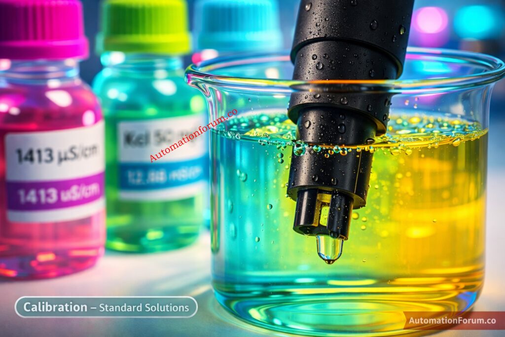
ISO Instrument Calibration Audits in Process Industries
In modern process industries, instrument calibration is one of the most important things to do to make sure quality. Instrumentation that works well is very important for plants that work in the oil and gas, petrochemical, power generating, pharmaceuticals, fertilizer manufacture, and water treatment industries. Field instruments that are connected to PLC, DCS, and safety systems constantly check and control process parameters like pressure, temperature, flow, level, and analytical composition.
The results can be very bad if these tools give wrong measurements. Incorrect readings may lead to process instability, product quality issues, environmental violations, or even major safety incidents. For example, an improperly calibrated pressure transmitter in a boiler system could cause incorrect control actions that lead to overpressure conditions.
As part of their quality management systems, firms use organized ISO calibration audit procedures to make sure that their measurements are accurate and meet international standards. An instrument calibration audit checklist helps verify whether measuring equipment is properly calibrated, traceable to national standards, and maintained according to documented procedures.
ISO internal audits are very significant in process plants because they help companies find calibration problems before external certification audits or regulatory inspections. A well-implemented ISO internal audit instrumentation program makes sure that measurements are accurate, that they can be traced, and that all production processes follow the rules.
An ISO instrument calibration audit is a planned check of the organization’s measurement and calibration processes to make sure they follow both international standards and the organization’s own rules.
Objectives of Calibration Verification in Process Plants
The audit checks to see if the tools used to monitor and control processes are properly calibrated, can be traced back to known measurement standards, and are managed through a structured calibration system.
Importance of Measurement Traceability in Industrial Calibration
Calibration audits usually check to see if a company is following a number of ISO standards that deal with quality management and measurement systems.
Key ISO Standards for Process Instrument Calibration
ISO 9001 Requirements for Calibration of Measuring Equipment
This is the standard for quality management systems around the world. It requires businesses to make sure that the measurement tools they use to check if a product meets standards are calibrated or checked at set times using standards that can be traced.
ISO IEC 17025 Calibration Laboratory Competence Standard
This standard defines the competence requirements for calibration and testing laboratories. Calibration laboratories accredited to ISO 17025 demonstrate their ability to produce technically valid calibration results.
ISO 10012 Measurement Management System Requirements
ISO 10012 provides requirements for establishing a measurement management system that ensures measurement processes and equipment deliver reliable and traceable results.
ISO 14253 Measurement Verification and Uncertainty Rules
This standard focuses on verification of measuring equipment and decision rules related to measurement uncertainty.
These standards work together to make up the basis for calibration audit instrumentation systems used in factories.
Why Internal Calibration Audits are Critical in Process Plants
In process industries, internal calibration audits are very significant since measuring systems have a direct impact on the safety of the plant, the quality of the products, and the reliability of the operations.
In manufacturing, measurements can be done at different times, but in process plants, measurement equipment must work all the time, 24 hours a day.
Any change in an instrument can have an instantaneous effect on how well the plant works.
DCS and PLC platforms are examples of advanced process control systems that modern process facilities use. These systems control pumps, valves, compressors, and reactors using sensor data in real time.
Temperature sensors that control the heating zones in a furnace
If these instruments drift out of calibration, the control system will respond incorrectly, potentially causing process instability or equipment damage.
Safety Instrumented Systems and Emergency Shutdown Sensors
Reliable sensors are very important for safety systems.
For example:
High pressure shutdown transmitters
Emergency shutdown switches
Flame detectors
Gas detectors
If these tools are not set up appropriately, the Safety Instrumented System (SIS) might not go off when there is a dangerous condition.
Calibration audits therefore play a direct role in plant safety management.
Custody Transfer Measurement Accuracy in Oil and Gas Plants
In oil and gas industries, many instruments are used for custody transfer measurement where product quantities are measured for financial transactions.
Scope of Calibration Audit in Process Instrumentation
A calibration audit in process industries usually includes all of the measuring and monitoring tools that affect the operation of the process, safety, product quality, and compliance with environmental laws.
Process Instruments Typically Included in Calibration Audits
Process plants use a wide range of field instruments that must be included in calibration programs.
Pre Audit Preparation for ISO Instrument Calibration Audit
To do an internal calibration audit well, you need to be well-prepared. If auditors don’t prepare well enough, they could miss important problems or not look at important parts of the calibration system.
Verification of Instrument Master List and Database
The first thing to do is check the instrument master database.
This list should have:
Instrument tag number
Instrument type
Location
Calibration frequency
Last calibration date
Next calibration due date
Instrument criticality classification
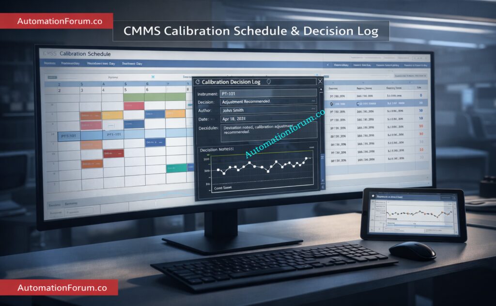
CMMS or asset management systems usually keep the instrument master list up to date.
Review of Calibration Schedule and Overdue Instruments
Auditors need to check that calibration schedules are being followed correctly.
The review should find:
Overdue instruments
Instruments approaching calibration due date
Instruments removed from service
Spare instruments stored in warehouse
This stage helps find problems with the schedule before the audit starts.
If a technician uses a calibrator that has expired, all of the measurements made with that device are no longer reliable.
Missing Measurement Traceability Documentation
One of the most important ISO requirements is measurement traceability. It must be possible to trace calibration results back to known national or international measuring standards.
Not being able to keep track of things is a big problem that auditors notice.
Poor Instrument Tagging and Identification
Some plants may have broken, missing, or unreadable instrument tags.
Auditors can’t connect instruments to calibration records without the right identification.
Best Practices for Maintaining ISO Calibration Compliance
To be in conformity with ISO calibration, you need to do more than just calibrate your equipment every so often. It needs a well-organized and well-managed system for taking measurements.
Digital Calibration Management Systems for Process Plants
Calibration management software that works with CMMS platforms is used in modern plants.
For example:
SAP PM
Maximo
Asset management systems
Calibration management databases
These technologies assist keep track of calibration history and make scheduling easier.
Risk Based Calibration Interval Management
Not all instruments need to be calibrated at the same time.
Instruments that are really important should have shorter intervals, while instruments that are not very important might have larger intervals.
Risk-based approaches assist make the best use of maintenance resources.
Instrument Criticality Classification Methods
Instruments should be classified according to their effect on:
Safety
Environment
Product quality
Production efficiency
During audits and planning for maintenance, critical tools are given priority.
Automated Calibration Notifications and Scheduling
Automated notifications assist technicians find devices that are getting close to their calibration due dates.
This lowers the chance of instruments being late.
Calibration Document Control and Record Management
Calibration procedures, calibration records, and traceability certificates must be maintained under strict document control systems.
This ensures that technicians always use the latest procedures.
Internal Audit Checklist for Instrument Calibration in Process Industries
For the plant to run safely and reliably, it is important to keep the process instrumentation correct. In the oil and gas, petrochemical, power generation, pharmaceutical manufacturing, and water treatment industries, thousands of instruments are always measuring things like pressure, temperature, flow, level, and analytical data. If these tools aren’t set up appropriately, the facility could have problems with process stability, product quality, not following the rules, or even safety.
Engineers can use an instrument calibration internal audit checklist to make sure that calibration activities are always in line with ISO standards and factory procedures.
An instrument calibration internal audit checklist helps engineers systematically verify whether calibration activities meet ISO requirements and plant procedures. This checklist supports ISO 9001 calibration compliance, ensures measurement traceability, and helps auditors evaluate calibration procedures, records, technician competency, and calibration equipment traceability.
The following detailed ISO calibration audit checklist is designed for:
It provides a structured method to audit calibration management systems, calibration procedures, calibration equipment, documentation, traceability, and non-conformance handling.
A calibration audit is a systematic review of calibration procedures, records, and equipment to verify compliance with quality standards. It confirms that measurement instruments are accurate and properly maintained.
Why is calibration important in process industries?
Calibration ensures that instruments measure process parameters accurately, preventing process deviations and safety risks. Regular calibration also maintains product quality and regulatory compliance.
What is traceability in calibration?
Traceability means measurement results can be linked through an unbroken chain of calibrations to national or international standards. This ensures measurement reliability and consistency.
Which ISO standards apply to instrument calibration?
Common standards include ISO 9001 for quality management, ISO 17025 for calibration laboratories, and ISO 10012 for measurement management systems. These standards define how calibration systems should be managed.
How often should process instruments be calibrated?
Calibration frequency depends on instrument criticality, manufacturer recommendations, and plant risk assessment. Most industries follow annual or semi annual calibration intervals.
What is an instrument calibration audit checklist?
It is a structured list of audit questions used to verify calibration procedures, records, traceability, and compliance with ISO requirements. It helps auditors evaluate the effectiveness of calibration systems.
What documents are reviewed during a calibration audit?
Auditors review calibration certificates, instrument master lists, procedures, traceability records, and technician training documents. These records demonstrate compliance with calibration standards.
What happens if an instrument is found out of calibration?
The instrument must be adjusted or recalibrated, and previous measurement results may need to be evaluated for impact. Corrective actions should be documented in the audit records.
Who performs internal calibration audits?
Trained ISO internal auditors, quality engineers, or instrumentation specialists within the company usually do internal calibration audits.
What instruments require calibration in process plants?
Pressure transmitters, flow meters, temperature sensors, level transmitters, analyzers, and control valves are all common tools. Calibration should be done on any equipment that is used to measure or keep an eye on something.
What is the purpose of calibration records?
Calibration records show that instruments were calibrated appropriately and are still within acceptable tolerance limits. These records help with compliance with ISO and tracking.
What are common findings in calibration audits?
Common problems include missing calibration records, expired calibration certificates, wrong processes, and not being able to trace measurements. When ISO audits happen, these problems can cause things to not be in compliance.
Can calibration be done in house?
Yes, companies can calibrate things in-house as long as they have qualified staff, the right protocols, and reference standards that can be traced. We employ outside authorized labs when we need more accurate results.
What is the difference between calibration and verification?
Calibration checks an instrument against a reference standard to find out how much it is off. Verification just makes sure that the instrument works within acceptable limitations.
How does calibration support ISO certification?
Regular calibration shows that measuring tools give accurate results and meet ISO quality management standards. This helps with successful ISO audits and getting certified.
Refer the below link for the Free Instruments Calibration Procedures: 60+ Step-by-Step Methods for Pressure, Temperature, Flow & Level
Why Oxygen Analyzers are Critical in Power Plants and Process Industries
Power plants, refineries, and chemical process industries all need oxygen analyzers to keep an eye on combustion efficiency, safety, and environmental compliance. Instrumentation and control engineers need to know how paramagnetic, zirconia, and electrochemical oxygen analyzers function, as well as how to properly sample, install, and calibrate them.
Enhance Oxygen Analyzer Expertise for Instrumentation and Control Engineers
Improving your understanding of sample conditioning, signal integration (4–20 mA, HART), and fixing problems such sensor drift, poor response, and contamination helps make sure that oxygen measurements are precise and process control is reliable in industrial settings.
This difficult 25-question quiz is for experienced instrumentation and EPC process engineers. It tests their practical understanding of oxygen analyzers used in process industries. It checks things like operating principles (paramagnetic, zirconia, electrochemical, infrared), sampling and conditioning, installation and probe positioning, calibration, signal integration, troubleshooting, safety, computations, and validation. You should expect scenario-based and mathematical challenges that are similar to what happens in real plants.
Use this quiz to find out what technicians don’t know, reinforce proper practices, and get them ready for field commissioning and audits. After each question, there are detailed answers and time estimates to help with focused study and use on the job. Great for training sessions, checking skills and getting ready for ongoing professional growth.
Advanced 25-Question Oxygen Analyzer Quiz for Instrumentation Engineers
Calibration vs Verification: a Commonly Confused Concept
Calibration and verification are often confused by instrumentation engineers, calibration professionals, quality managers, and technical authors that work in process industries. Both exercises are about making sure measurements are correct, but they have different goals and follow different steps. Not knowing the difference can cause problems with compliance, bad process control, and expensive operational concerns.
In fields like oil and gas, petrochemical plants, electricity generation facilities, fertilizer production units, and chemical processing plants, safety, product quality, and following the rules all depend on how accurate measurements are. Because of this, businesses need to make sure they know the difference between calibration and verification and employ each one correctly in their instrumentation management programs.
This article explains the concept of calibration and verification in clear and practical terms. It provides definitions, comparisons, real industrial examples, procedures, common mistakes, and best practices so instrumentation professionals can confidently apply the correct approach in their daily work.
Why Understanding the Difference Between Calibration and Verification Matters In Process Industries
Impact Of Measurement Accuracy On Industrial Process Control
Accurate measurements are the foundation of process control systems. Instruments such as pressure transmitters, flow meters, temperature sensors, and weighing systems provide the critical data used by control systems to regulate industrial processes.
Risks Of Incorrect Instrument Measurements
When these instruments drift or provide incorrect readings, several problems can occur. Conditions in the process may go outside of the range they were meant to work in. Safety interlocks might not work right. The quality of the product may not meet the standards. In businesses that are regulated, wrong measurements can potentially cause compliance problems during audits.
Both calibration and verification are used to make sure that measurements are accurate, although they are employed for different things.
Role Of Calibration And Verification In Regulatory Compliance
Using traceable standards, calibration finds out how accurate an instrument really is.
Verification just makes sure that the instrument is still working within a range of allowable tolerances.
Knowing when to use each method helps plants keep accurate readings without having to do extra calibration work, while still making sure they follow the rules and are reliable.
Calibration is a controlled way to compare the output of an instrument’s measurement to a recognized reference standard whose value is known and can be traced back to national or international standards.
Purpose of Calibration in Industrial Measurement Systems
The goal of calibration is to find out how the instrument reading and the reference standard’s true value are related. If the instrument doesn’t indicate the right value, you can make changes to get the measurement inside the permitted range.
Key Elements of A Proper Calibration Process
Calibration normally means taking measurements at several points across the instrument’s entire operational range. This makes sure that the instrument works appropriately at all three levels of measurement: low, mid, and high.
A proper calibration process typically includes the following elements.
Comparison with a traceable reference standard
Multiple test points across the instrument range
Measurement of deviation or error
Adjustment if necessary
Calculation of measurement uncertainty
Documentation in the form of a calibration certificate
Calibration records are usually stored in calibration management systems or maintenance databases and are often required during quality audits.
Calibration establishes measurement traceability and provides documented proof that the instrument is capable of producing accurate readings.
Verification is a simpler activity performed to confirm that an instrument is functioning correctly within a specified tolerance.
Verification usually only verifies one or two measurement points with a reference device instead than doing a full multi-point calibration.
Purpose of Verification in Maintenance Programs
The purpose is not to find out how accurate the measurements are, but to make sure that the instrument hasn’t gone outside of permitted limitations.
People usually do verification between specified calibration times or after maintenance work.
Typical Characteristics of Instrument Verification
Typical characteristics of verification include the following.
Limited measurement points such as zero and mid range
Pass or fail assessment
Minimal documentation compared to calibration
Faster procedure requiring less downtime
Often performed by plant technicians or operators
If the instrument passes verification, it continues to remain in service until the next scheduled calibration. If the instrument fails verification, a full calibration or repair is usually required.
Verification therefore acts as an early warning check that helps detect potential measurement drift before it becomes a serious problem.
Key Differences Between Calibration and Verification
Calibration and verification both have to do with making sure that instruments are accurate, but they are used for distinct things in industrial measuring systems.
Purpose and Objective Differences
Calibration is a thorough process that compares an instrument’s findings to traceable reference standards to find out how accurate its measurements really are. It requires testing the instrument at several places along its working range and writing down the results in a calibration certificate.
Verification, on the other hand, is a simpler way to check that an instrument is still working within an acceptable range. It usually involves checking one or two measurement points and determining whether the instrument passes or fails the test.
Measurement Method Differences
Calibration establishes measurement traceability and provides documented evidence of accuracy. Verification provides a quick confirmation that the instrument has not drifted significantly since the last calibration.
Understanding these differences helps engineers maintain reliable instrumentation systems while avoiding unnecessary calibration work.
Practical Industrial Examples of Calibration Vs Verification
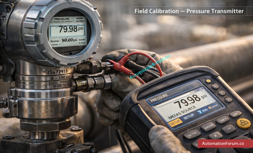
Pressure Transmitter Calibration And Verification Example
Calibration of a pressure transmitter normally involves isolating the transmitter from the process and connecting it to a precision pressure calibrator or dead weight tester. Pressure values are applied at several points such as zero percent, twenty five percent, fifty percent, seventy five percent, and one hundred percent of the transmitter range.
The technician records both the applied pressure and the transmitter output signal. If the transmitter output deviates from the expected value, adjustments are performed to correct the zero and span settings.
Verification of a pressure transmitter may involve applying a single pressure value using a portable pressure calibrator. The technician checks whether the transmitter output signal matches the expected value within the acceptable tolerance. If the measurement is within limits, the transmitter passes verification.
Calibration of flow meters such as turbine or magnetic flow meters typically requires specialized calibration facilities or flow laboratories. Water or another calibration fluid is passed through the meter at several controlled flow rates, and the measured output is compared with the reference flow measurement.
Verification of a flow meter may involve comparing its reading with a portable clamp on ultrasonic flow meter or comparing process readings with another trusted reference meter.
Temperature Sensor Calibration and Verification Example
Calibration of temperature sensors such as RTDs or thermocouples is usually performed using a dry block calibrator or liquid bath. The sensor is tested at multiple temperature points and compared with a certified reference thermometer.
Verification may involve comparing the sensor reading with a portable temperature indicator at one process temperature point to confirm the sensor has not drifted significantly.
Weighing Balance Calibration Vs Verification Example
Calibration of a weighing balance uses certified standard weights traceable to national measurement standards. The balance is tested at multiple weight levels to evaluate linearity and repeatability.
Verification may involve placing a routine check weight on the balance to confirm that the displayed value remains within the allowable tolerance.
Preparation begins with identifying the instrument tag number, serial number, and calibration history. The technician selects appropriate reference standards and verifies that their calibration certificates are valid.
The instrument is then isolated from the process and connected to the calibration reference device. Safety precautions such as lockout procedures and work permits are followed when necessary.
Reference values are applied across the measurement range. At each point the instrument output is recorded and compared with the reference value.
Measurement errors are calculated and analyzed. If the instrument exceeds the acceptable tolerance, adjustments are performed.
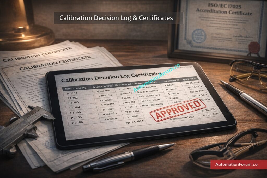
Once the instrument performs within specification, the calibration results are documented. A calibration certificate is generated containing information such as instrument identification, calibration date, reference standards used, measurement results, technician name, and next calibration due date.
Finally the instrument is labeled with a calibration sticker and the calibration record is updated in the maintenance or calibration management system.
Complete Calibration Guide for Level Measurement Devices:
The technician first confirms the instrument identification and obtains a portable reference device that has a valid calibration status.
The reference value is applied to the instrument at one or two predetermined points. The instrument reading is compared with the reference measurement.
If the instrument reading falls within the acceptable tolerance range, the instrument passes verification and continues operating.
If the instrument fails the verification check, the instrument is scheduled for full calibration or removed from service depending on its criticality.
Verification results are recorded in a logbook or maintenance system along with the date, technician name, reference device used, and pass or fail result.
Many industries operate under strict quality and measurement control requirements. Calibration activities are often governed by quality management standards and industry regulations.
International laboratory competence requirements are defined by the standard ISO/IEC 17025. This framework ensures that laboratories performing calibration services maintain traceability to national measurement standards and follow documented quality systems.
Quality Management and Measurement Traceability
Process industries also follow internal calibration procedures aligned with regulatory frameworks, manufacturer recommendations, and plant risk management practices. Maintaining proper calibration documentation helps organizations demonstrate measurement reliability during audits and inspections.
Common Mistakes When Performing Calibration and Verification
Using Uncalibrated Reference Instruments
One common mistake is assuming that a quick verification check is equivalent to calibration. Verification only confirms that the instrument appears to be functioning correctly at a specific point. It does not establish complete measurement accuracy across the entire range.
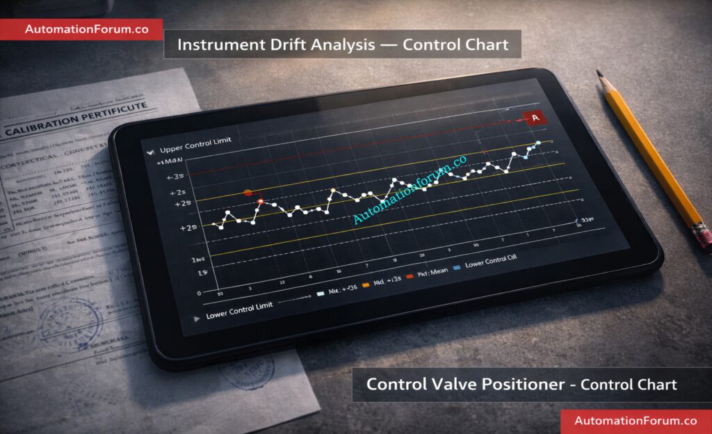
Ignoring Historical Calibration Drift Data
Another frequent issue is using reference instruments that are themselves out of calibration. If the reference device is inaccurate, the verification or calibration result becomes unreliable.
Some organizations also fail to review calibration trends. Over time, instruments may show gradual drift. Without analyzing historical calibration data, this drift may remain unnoticed until it causes process problems.
Poor Calibration Documentation Practices
Poor documentation is another problem. Missing calibration certificates, incomplete records, or inconsistent documentation formats can create serious difficulties during audits.
Clear procedures, proper training, and consistent documentation help eliminate these problems.
Industrial Case Study: Consequences Of Relying Only on Verification
Problem in Reactor Temperature Measurement
A petrochemical plant relied heavily on verification checks for its temperature transmitters in a reactor control system. Operators regularly compared transmitter readings with local indicators and recorded them as acceptable.
However, during a scheduled calibration shutdown, technicians discovered that several transmitters had gradually drifted by more than two degrees Celsius. Because verification checks were performed only at a single operating temperature, the drift at other temperature levels went unnoticed.
Impact on Process Performance
The incorrect temperature readings caused the reactor control system to operate outside its intended range, affecting product yield and increasing energy consumption.
Corrective Actions Implemented by the Plant
Following the incident, the plant revised its instrumentation maintenance procedures. Full multi point calibration intervals were maintained, and verification checks were expanded to include multiple operating points. Calibration trend analysis was also introduced to detect measurement drift earlier.
This case demonstrates that verification alone cannot replace proper calibration.
Calibration should be performed under several conditions to ensure measurement reliability and compliance with industrial standards.
Calibration is typically required when an instrument is newly installed in the plant. New instruments must be calibrated before being placed into service to confirm their measurement accuracy.
Calibration should also be performed after instrument repair or major maintenance activities. Any adjustment or component replacement may affect measurement accuracy.
Scheduled calibration intervals are another important factor. Many plants perform calibration annually or semi annually depending on instrument criticality and process requirements.
Calibration is also required when a verification check fails. If an instrument does not meet the acceptable tolerance during verification, a full calibration must be performed to determine the actual measurement error.
In regulated industries, calibration may also be required to meet quality standards and audit requirements.
Verification is usually performed between calibration intervals to confirm that instruments are still functioning correctly.
Routine verification checks can be performed during maintenance inspections or process shutdowns. These checks help detect measurement drift early without performing a full calibration.
Verification may also be performed after minor maintenance activities such as replacing cables, reconnecting transmitters, or cleaning sensors.
Another common use of verification is during troubleshooting. Engineers may verify an instrument reading using a portable reference device to determine whether a process issue is caused by instrumentation or by actual process conditions.
Because verification procedures are faster and simpler, they allow technicians to monitor instrument health without interrupting plant operations for long periods.
How Calibration Frequency is Determined in Industrial Plants
Determining the correct calibration interval is an important part of an instrumentation maintenance program.
Several factors influence calibration frequency in industrial plants.
Instrument criticality is one of the most important considerations. Instruments involved in safety systems, custody transfer measurement, or regulatory reporting usually require more frequent calibration.
Manufacturer recommendations also provide guidance on typical calibration intervals for different types of instruments.
Historical calibration data is another valuable factor. If an instrument continuously exhibits minimal drift, the calibration interval may be prolonged. On the other hand, instruments that drift a lot may need to be calibrated more often.
Environmental factors like vibration, temperature changes, humidity, and corrosive surroundings can also make instruments less stable and need to be calibrated more often.
Plants can create risk-based calibration schedules that keep measurements accurate while making the best use of maintenance resources by looking at these aspects.
For industrial facilities to have reliable instrumentation systems, calibration and verification are both very important.
Calibration uses traceable reference standards to find out how accurate an instrument really is and creates a written calibration certificate.
Verification is a simple pass-or-fail test that makes sure an instrument stays within permissible parameters between calibration periods.
Calibration usually means taking measurements at several sites along the instrument’s range, while verification usually simply checks one or two points.
Both of these things work together to make sure that measurements are accurate, products are of high quality, and process industries follow the rules.
Why Calibration and Verification are Both Critical for Process Industry Measurement Systems
An successful instrumentation maintenance program must include both calibration and verification. Even though they have diverse jobs, they all work together to make sure that measurement systems stay precise, dependable, and in line with industry standards.
Calibration gives you proof that your measurements are accurate by doing extensive multi-point tests and keeping records. Verification is a quicker way to make sure that instruments stay within acceptable operating parameters between calibration intervals.
Organizations can avoid expensive measurement mistakes and keep trust in their instrumentation systems by explicitly outlining these tasks in plant procedures, teaching staff on the right way to execute them, and keeping good records.
Knowing the difference between calibration and verification will help you regulate your processes better, make your products better, and follow industrial standards more closely.
Frequently Asked Questions (FAQ) on Calibration vs Verification
What is the difference between calibration and performance verification?
Calibration compares an instrument with a traceable reference standard to determine measurement error and establish accuracy. Performance verification simply checks whether the instrument still meets specified performance limits without full calibration.
Can I do a verification instead of calibration to save time?
Not if traceability, uncertainty, or regulatory compliance is required. Verification is a quicker interim check; calibration is required at scheduled intervals or after repair, or when legal/quality traceability is needed.
How often should calibration be done?
Frequency depends on instrument criticality, manufacturer guidance, process risk, stability history, and regulatory requirements. Use data (trend analysis) to set intervals rather than arbitrary dates.
Who can perform calibration vs verification?
Calibration should be performed by qualified calibration personnel or accredited labs. Verification can be performed by trained operators or technicians following a documented procedure.
Does calibration always require adjustment?
Calibration documents the error. If the error is within acceptable uncertainty, no adjustment may be necessary. If it exceeds limits, adjustment or repair is required.
What is measurement uncertainty and why is it important?
Uncertainty quantifies the doubt in a measurement result. It’s essential in calibration to determine whether an instrument truly meets required specifications when uncertainty is considered.
What is the difference between control and calibration?
Calibration makes assurance that measurements are correct by comparing an instrument to a known reference standard. Control is the regular monitoring that makes sure readings stay steady and consistent over time.
What is the difference between equipment calibration and validation?
Calibration of equipment makes ensuring that an instrument measures correctly against known standards. Validation demonstrates that a system or equipment consistently performs its intended function within the required process conditions.
What is the difference between calibration and verification?
Calibration determines measurement accuracy using traceable standards and produces documented calibration results. Verification checks whether the instrument output falls within a defined tolerance without performing full calibration.
What are the four types of calibration?
Common calibration categories include electrical calibration, mechanical or dimensional calibration, temperature calibration, and pressure or flow calibration. These categories are based on the measurement parameter and the type of industrial instrument being tested.
The ISO Rules Every Instrument Engineer Should Know: ISO Standards For Instrumentation Calibration Complete Guide for Industrial Engineers
Reliable signal transmission is very important for accurate measurement and consistent control in today’s industrial automation systems. Instruments including transmitters, analyzers, control valves, PLC systems, and distributed control systems (DCS) are very important for process facilities to keep an eye on and control their operations. These instruments work with very weak signals, and even tiny electrical problems might cause measurement mistakes or make process control unreliable.
Instrument Earth (IE) is a vital way to keep signals accurate and safeguard instrumentation equipment from electrical noise. Some people call Instrument Earth Electronic Earth, Clean Earth, Reference Earth, or Signal Earth. Its main job isn’t to keep people from getting shocked by electricity; it’s to make sure that sensitive electronic equipment used in measurement and control systems has a steady electrical reference.
Instrument Earth (IE) is a special grounding system for control and instrumentation equipment. It provides a stable reference potential for electronic circuits that handle measurement and communication signals.
Most instrumentation signals in process industries operate at low energy levels. Examples include:
4–20 mA analog signals
HART communication signals
Digital input and output signals
Fieldbus communication networks
Analyzer measurement signals
Because these signals operate at very small voltage or current levels, they are vulnerable to electrical interference. If electrical noise enters the signal path, it can distort measurements and cause incorrect process control decisions.
Instrument Earth helps prevent this by maintaining a clean and stable reference point for all instrumentation equipment.
Why Instrument Earth Matters in PLC and DCS Systems
How Instrument Earthing Improves Measurement Accuracy
Industrial plants contain many sources of electrical interference. Large motors, variable frequency drives, transformers, welding machines, and power cables generate electromagnetic noise that can couple into instrumentation cables.
Without a proper earthing system, this noise may enter measurement circuits and create several operational problems.
Impact on Control Loop Stability and Communication Reliability
Some common problems that happen when earthing isn’t done well are:
Inaccurate measurements: Electrical noise can change the shape of analog signals, like 4–20 mA loops. A slight adjustment can modify the temperature, pressure, flow, or level that is being measured.
Error in communication: Modern instruments talk to each other using digital protocols like Fieldbus, Modbus, or HART. These signals can get messed up by electrical interference, which can lead to communication problems.
Control loops that aren’t stable: If noise causes measurement signals to change, the control system might not work right. This can make control loops oscillate and processes run in an unpredictable way.
Unexpected equipment trips: Alarms or safety shutdowns may go off even when the operation is running smoothly if the indications are wrong.
Instrument Earth lowers these dangers by giving instrumentation equipment a separate, low-noise grounding reference.
Instrument Earth (IE) vs Safety Earth (PE) – Key Differences
There are two types of grounding systems used in industrial plants: Instrument Earth and Safety Earth. They are not the same thing.
Safety Earth keeps humans from getting shocked by electricity, and Instrument Earth keeps sensitive instrumentation signals safe from noise and interference.
Common Noise Sources (Motors, VFDs, Welding, Lightning)
Industrial settings are electrically loud because a lot of electrical and electronic gadgets create electromagnetic interference (EMI) that can mess with signal transmission and instrumentation systems.
These devices create powerful electromagnetic fields that might cause unintended voltages to appear in neighboring instrumentation connections.
These induced voltages can cause signal distortion, unstable readings, communication problems, and wrong process measurements in control systems like PLC or DCS if they are not properly shielded, routed, grounded, and instrument earthed.
Give the instrument its own ground, independent from the power ground. This dedicated earth keeps a low-noise reference for sensitive signals and stops power fault currents from messing up measurements.
Make sure that all of the instruments have the same ground reference. When transmitters, sensors, and I/O modules all use the same reference, measurement offsets and common mode errors are less likely to happen.
Controlled single point bonding can help you avoid ground loops. If you have to make more than one connection, employ isolation or bonding methods that keep currents from flowing across signal shields.
Correctly connect the cable shields to the instrument ground. Proper termination routes captured interference to earth instead of into signal conductors.
Use low resistance, short bonding leads. Short direct bonds between shields chassis and the instrument earth bus reduce loop area and lower induced noise.
Route instrument earth conductors away from power runs. Physical separation from motors VFD runs and power trays reduces electromagnetic coupling and induced voltages.
Centralize instrument earth in marshalling or control cabinets. An instrument earth bus bar inside the cabinet provides a single tidy point for shield and chassis terminations.
Connect cable shields chassis and signal returns to the same earth bus. This ensures I/O modules receive consistent reference voltages and avoids measurement drift.
Size grounding conductors so that they have low impedance even when the conditions are changing. When there are strong transient currents elsewhere in the plant, proper sizing keeps potentials steady.
Don’t share earth routes with power cables that carry a lot of current. Shared routes can add noise to the control system and mess with both analog and digital I/O.
Use isolation modules when long runs risk loop formation. Signal isolators maintain accuracy without breaking safety or overall bonding requirements.
Label earth terminals clearly for maintenance and testing. Clear labeling prevents accidental cross connections that reintroduce loops or noise.
Cable Shielding and Shield Termination Best Practices
Use continuous shields with a reliable drain conductor. A continuous shield intercepts external fields and drain wires provide a consistent connection to instrument earth.
Terminate shields at the appropriate end according to project rules. Single end termination at the control room is common to avoid creating a shield current path that forms a loop.
Prefer individual pair shields for low level analog pairs. Separate shields reduce crosstalk and protect microvolt level signals better than an overall shield alone.
Use overall shields for long multipair trunk cables. Overall shields protect grouped signals during long runs from junction boxes to the control room.
Inspect shield continuity and bond quality during commissioning. Poor shield continuity is a common root cause of EMI problems and must be verified with tests.
Avoid bonding shields to random structural steel or piping. Bonding to arbitrary metal can create unpredictable noise paths and upset instrument references.
Typical Instrument Earth System Arrangement (Field → Control Room)
Field instruments connect to local junction boxes then to trunk cables. This staged routing collects signals while preserving shield continuity and ease of maintenance.
Trunk cables terminate in marshalling panels or control cabinets. Inside these enclosures shields and chassis grounds meet the instrument earth bus.
Instrument earth bus links to the plant grounding grid at a controlled single point. Single point bonding helps control loop currents while still allowing a fault path to the main grid.
Dedicated earthing conductors carry the instrument earth to the main grid. These conductors should be routed separately from heavy current conductors.
Use signal isolators or common mode filters where layout or long runs demand. These devices help maintain signal integrity when perfect routing cannot be achieved.
Include the earthing topology in the as-built drawings. Keeping accurate records makes it easier to fix problems and stops people from making changes that make noise by unintentionally.
Inside PLC and DCS control panels, the instrument earth bus bar serves as the main grounding reference for instrumentation equipment.
Usually, this copper bus bar is installed within system cabinets or marshalling cabinets and connected to the plant’s grounding grid via special earthing conductors.
The instrument earth bus bar is a place where all of the following can connect:
Plan earthing and cable trays early on in the engineering process. Early planning avoids retrofits that are often noisy and expensive to correct.
Segregate instrument and power cable trays and avoid long parallel runs. Physical separation is one of the simplest and most effective noise reduction measures.
Terminate shields to designated instrument earth terminals only. Using designated terminals keeps shield drainage consistent and avoids ad hoc bonding.
Keep bonding leads short straight and mechanically robust. Long looping bonds increase susceptibility to induced voltages and may corrode over time.
Use corrosion resistant lugs and label all connections. Good mechanical connections preserve low resistance and make maintenance safe and quick.
Perform continuity and resistance checks after installation. Checking low resistance paths and shield continuity before commissioning stops a lot of problems from happening later.
Common Problems Caused by Poor Instrument Earthing
Analog readings that change and measurements that drift. Noise and common mode voltages can randomly alter reported values and upset control loops.
Communication failures and intermittent data loss. Induced interference on communication pairs causes retries packet loss and network instability.
False alarms, trips that come out of nowhere, and annoying shutdowns. Noise can make protective logic think that real process events are happening when they aren’t.
It is hard to find out what is wrong with intermittent issues. Ground-related problems generally go away on their own, which makes finding the main cause slow and expensive.
Repeated transients shorten the life of equipment. Repeated electrical stress speeds up the aging of parts and makes maintenance more frequent.
First, look at all of the shield and earth terminations. Loose corroded or miswired connectors are a frequent and easily fixed cause.
Measure continuity and resistance between instrument earth points. High resistance joints reduce noise drainage and should be corrected.
Use an oscilloscope or clamp meter to observe noise while equipment runs. Real time observation helps correlate noise with specific machines or events.
Re route suspect cables away from noisy sources and secure shields. Physical separation and correct shield termination often yield immediate improvements.
Install isolators common mode chokes or filter modules if needed. When routing fixes are impossible these devices reduce the effect of common mode interference.
Record measurements before and after changes. Documentation validates fixes and prevents reintroduction of problems by future work.
Design earthing as part of the system architecture not as an afterthought. Integrate trays earth bars and cabinet layouts into project specifications from day one.
Maintain consistent shield termination and bonding rules across the plant. Consistency keeps behavior predictable and troubleshooting straightforward.
Keep periodic inspection maintenance and re torque schedules. Regular checks catch corrosion and loosening before they impact operations.
Train technicians and engineers on correct earthing practices and documentation. Skilled staff prevent accidental rework that creates noise or unsafe conditions.
Maintain a log of grounding resistance and continuity tests. Trend data reveals degrading connections before they produce failures and supports proactive maintenance.
Refer the below link to read the Essential Earthing Drawing Guide
What is the difference between plant earth and instrument earth?
People utilize plant earth to keep equipment secure and guard against electrical shocks by safely transferring fault currents to ground.
Instrument earth gives sensitive instrumentation signals a clean reference ground so that measurements stay accurate.
How to check instrument earthing?
Instrument earthing is checked by inspecting grounding connections, cable shield terminations, and instrument earth bus bars. Engineers may also measure grounding continuity or resistance using an earth tester to confirm proper grounding performance.
Instrument earthing is done by connecting instrumentation equipment, cable shields, and control system chassis to a dedicated instrument earth bus bar. This bus bar is then connected to the plant grounding grid through a low-resistance earthing conductor.
What is the difference between electrical earthing and instrument earthing?
Electrical earthing protects persons and equipment by safely sending fault currents to the ground when there are electrical problems.
How often should Instrument Earthing systems be inspected?
Instrument earthing systems should be inspected periodically as part of routine plant maintenance programs. Regular inspections ensure grounding connections remain secure, corrosion-free, and effective in reducing electrical noise.
Are Instrument Earth and Safety Earth connected together?
Instrument Earth and Safety Earth are normally routed separately within industrial plants to prevent electrical interference. However, they are typically bonded together at a single point in the main plant grounding grid.
What problems can occur if Instrument Earth is not installed properly?
Improper instrument earthing can cause fluctuating analog signals, unstable control loops, and communication errors in PLC or DCS systems. It may also lead to false alarms, unexpected equipment trips, and unreliable process measurements.
Should cable shields be connected to Instrument Earth?
Yes, cable shields in instrumentation cables should normally be connected to the Instrument Earth system. This allows electromagnetic noise captured by the shield to be safely drained to ground, protecting sensitive signal circuits.
Ensure Signal Integrity with Proper Instrument Earthing
Instrument Earth is a fundamental part of industrial automation systems. While Safety Earth protects people from electrical hazards, Instrument Earth protects the accuracy and reliability of measurement and control signals.
In modern plants where automation systems depend on precise data from hundreds of instruments, even small electrical disturbances can affect operations.
Instrumentation systems depend on precise and stable signals from field devices. A properly designed instrument earthing system provides a clean electrical reference, reduces electromagnetic interference, and ensures reliable communication between field instruments and control systems. By following proper grounding practices, using shielded cables, and maintaining dedicated instrument earth connections, industrial plants can significantly improve automation system performance and operational reliability.
One of the most crucial analytical measurements utilized in process industries like power plants, water treatment facilities, pharmaceutical plants, chemical industries, and food processing facilities is liquid conductivity measurement. To ascertain the purity, concentration, and degree of contamination of liquids, conductivity analyzers are frequently utilized.
It can be difficult to comprehend the electrical properties of conductivity probes, though. When choosing, setting up, or debugging conductivity analyzers, instrument engineers frequently have to compute probe resistance, total circuit impedance, and temperature-corrected conductivity values.
We have created a Conductivity Liquid Analyzer Probe Resistance Calculator to make this procedure easier. It uses your input parameters to automatically determine the values of resistivity, temperature-compensated conductivity, circuit impedance, probe resistance, and TDS.
Engineers can rapidly assess conductivity probe performance without doing calculations by using the calculator that is integrated into this page. It is intended especially for automation specialists, process engineers, calibration technicians, and instrumentation engineers who work with liquid analysis systems.
Conductivity Probe Resistance Calculator for Liquid Analyzers – Instrumentation Tool
⚡
Conductivity Liquid Analyser Probe
Resistance Calculation Smart Tool
🔧 AUTOMATIONFORUM.CO
Your Trusted Source for Automation Power Tools & Solutions
💧
µS/cmInput
🌡️
°CRange: -10 to 200
📈
%/°CCorrection Rate
📏
Range: 0.001 to 200 cm⁻¹
🔌
ΩWire Loss
📡
📊 CALCULATED RESULTS
⚡ Probe Resistance
—
Ω (at process temp)
🌡️ At 25°C
—
Ω (compensated)
📈 Total Circuit
—
Ω (Rl+Rc+Rp)
💧 Conductivity @ T
—
µS/cm
📡 Impedance |Z|
—
Ω
⚠️ Loading Error
—
%
🔬 Resistivity
—
MΩ·cm
🧂 TDS (approx)
—
mg/L
📐 Formulas
Rl = K / σ(T) = K / (σ₂₅ × [1 + α × (T − 25)] × 10⁻⁶)
Enter values above to compute
Refer the below link for the Ultimate Guide to Conductivity Transmitter Calibration Using a Decade Resistance Box:
When an AC voltage is put between the electrodes, ions in the solution conduct the current. The analyzer figures out the conductivity by measuring this current.
Conductance is the opposite of resistance, and it is the electrical property of the liquid that was measured.
Conductivity is calculated using the formula:
Conductivity = Cell Constant / Resistance
Where:
Cell Constant (K) represents electrode geometry
Resistance (R) is measured across electrodes
Top 25 Liquid Analyzer Interview MCQs Every Instrument Technician Must Know: Top 25 Essential MCQ for Liquid Analyzer Instrument Technician Interview in Process Industries
Why Temperature Compensation is Required
Temperature has a big effect on how well conductivity is measured.
When the temperature goes up:
Ion mobility increases
Electrical conductivity increases
Because of this, conductivity measurements are set to 25°C.
To get the right values for probe resistance, conductivity at process temperature, and other electrical properties of the measurement loop, the calculator needs the following inputs. These characteristics are the most important ones that affect how conductivity is measured in industrial liquid analysis equipment.
Conductivity at 25°C
This is the conductivity value of the solution at the standard temperature of 25°C. To keep results consistent across diverse conditions, conductivity values are usually compared to this temperature.
Typical ranges:
Ultrapure water: 0.055 µS/cm
Drinking water: 200–800 µS/cm
Seawater: ~50,000 µS/cm
Process Temperature
The temperature of the liquid that is being measured. Temperature has a big effect on conductivity because as the temperature goes up, ions move more easily, which makes it easier for electricity to flow through the solution.
Temperature Coefficient (α)
This number tells you how much conductivity changes for every degree Celsius. It shows how fast conductivity changes when the temperature changes.
Typical values:
Natural water: ~2% / °C
Chemical solutions: 1–3% / °C
Cell Constant (K)
This shows how the electrodes of the conductivity probe are shaped and sets the sensor's measurement range. Choosing the right cell constant makes ensuring that measurements are accurate for varied conductivity ranges.
Cable Resistance
Long cables between the conductivity probe and the analyzer add more electrical resistance to the measuring circuit. Adding cable resistance helps engineers figure out the total resistance of the circuit and any possible signal losses.
Excitation Frequency
To keep the measurement stable, conductivity analyzers use AC excitation signals to stop electrode polarization.
Typical excitation frequencies include:
60 Hz
1 kHz
3 kHz
10 kHz
With these inputs, the calculator can figure out how a probe would behave in the real world and calculate temperature-compensated conductivity, probe resistance, circuit impedance, and other electrical properties. This allows instrumentation engineers check the analyzer's settings, figure out how accurate the measurements are, and fix problems with conductivity measurement loops more easily.
The conductivity probe calculator gives instrumentation engineers a lot of important information that helps them better understand how to measure conductivity and how probes work electrically.
Probe resistance (process temperature)
The liquid's resistance between the probe electrodes at the process temperature. This number shows how much electrical resistance the conductive solution between the sensor electrodes has.
Resistance at 25°C
The temperature-compensated resistance value is based on the standard temperature of 25°C, which is often used as a reference point for measuring conductivity.
Total Circuit Resistance
It includes the resistance of the probe and the cable. This number helps engineers figure out the total resistance that the analyzer input sees and whether signal loading problems might happen.
Calculated automatically with temperature compensation. The calculator updates the conductivity value based on the temperature coefficient because conductivity changes with temperature.
Impedance (|Z|)
Takes into account both resistance and capacitive reactance. In systems that assess conductivity using AC excitation impulses, impedance is the total resistance to electrical current.
Resistivity
Resistivity is the opposite of conductivity. It is often used to measure ultrapure water, when very low conductivity levels are checked.
Total Dissolved Solids (TDS)
TDS is a rough estimate based on conductivity that shows how much dissolved material is in water.
Typical conversion:
TDS ≈ Conductivity × 0.64
The calculator gives these values right away, which lets engineers check the behavior of the probe, make sure the analyzer is set up correctly, and learn more about the electrical properties of conductivity measuring loops.
Conductivity at 25°C = 500 µS/cm Temperature = 40°C Temperature coefficient = 2% / °C Cell constant = 1 cm⁻¹
Step 1: Calculate Temperature Corrected Conductivity
σ(40) = 500 × [1 + 0.02 × (40 − 25)]
σ(40) = 500 × 1.3
σ(40) = 650 µS/cm
Step 2: Calculate Probe Resistance
Rl = 1 / (650 × 10⁻⁶)
Rl ≈ 1538 Ω
The conductivity calculator tool does this kind of math automatically, so engineers can rapidly find out the probe resistance and check the conductivity analyzer's performance without having to do the math themselves.
TDS stands for "total dissolved solids," which tells you how much dissolved material is in water.
How to test a conductivity probe?
Check the electrodes with your eyes and clean them. Then, dip the probe into approved conductivity standards (known µS/cm) and compare the reading to the standard. Also, check for stable readings at different concentrations and make sure that temperature correction is working.
What is the 4-probe method for measuring conductivity?
A four-electrode arrangement has two outer electrodes that send AC current and two interior electrodes that measure voltage. This gets rid of electrode polarization and contact resistance. Using the measured voltage and known current, you can find conductance. Then, using the cell constant, you can find conductivity.
What is the principle of a conductivity probe?
A conductivity probe sends an AC signal across electrodes. Ions in the solution carry the current, and the analyzer detects the current (or conductance). Using the probe's cell constant and temperature adjustment, conductivity is calculated from conductance.
What is the range of a conductivity probe?
The range depends on the cell constant and the design of the sensor. It can be as low as sub-µS/cm (for ultrapure water) to as high as tens of S/cm (for concentrated solutions). Depending on the probe you choose, the typical practical coverage is between 0.01 µS/cm and 50,000 µS/cm.
Is conductivity 1 resistance?
No, conductivity is not "one resistance." The opposite of resistivity is conductivity. Resistance depends on the shape and material. The cell constant connects conductivity (S/cm) and resistance (Ω) for probes: σ = K / R.
How to check temperature probe resistance?
Use a calibrated ohmmeter to check the sensor's resistance and see if it matches the expected resistance-vs-temperature curve (for example, PT100 = 100 Ω at 0°C). To be sure, measure at a known temperature (such in an ice bath or calibration bath) and check that the wiring and connectors are still working.
For keeping an eye on the quality of liquids in industrial operations, measuring conductivity is an important factor. For accurate conductivity analysis, you need to take into account things like the probe's shape, temperature correction, cable resistance, and analyzer input impedance.
Instrumentation experts can make dependable measurement systems and fix problems with conductivity analyzers better when they know these parameters.
The Conductivity Liquid Analyzer Probe Resistance Calculator makes these hard calculations easier and gives you fast results for probe resistance, impedance, resistivity, and temperature-compensated conductivity.
Engineers can easily check how conductivity probes work and make sure they work correctly in real-world situations with this tool.
Calibration Interval Scheduling in Process Industries
In industries that process things like oil and gas, petrochemicals, chemicals, fertilizers, and power generation, it is very important to accurately measure and regulate process variables so that operations can run safely and efficiently.
To make sure that measurements are accurate, process instrumentation like pressure transmitters, temperature sensors, flow meters, level instruments, analyzers, and control valves must be calibrated from time to time. However, calibrating at set times without taking into account how important the instrument is or how well it has worked in the past might lead to higher maintenance costs or more operational risk.
This method gives you an organized way to build a timetable for calibration intervals based on risk assessment, instrument importance, and past performance data. Plants may get the most out of their calibration frequencies while still making sure their measurements are accurate and follow the rules by using this strategy.
Purpose of the Calibration Interval Scheduling Procedure
This procedure’s goal is to set up a systematic way to develop and keep calibration interval schedules for process instrumentation.
This makes sure that:
Safe plant operation
Accurate process measurements
Compliance with regulatory standards
Reduced maintenance costs
Improved reliability of measurement systems
Instead of just following the manufacturer’s advice, you can find the best calibration frequency by looking at instrument drift, operational conditions, and criticality.
Scope of the Calibration Interval Procedure for Process Instrumentation
This protocol applies to all tools used in industrial process facilities for monitoring, control, and safety.
Risk-Based Method for Determining Calibration Intervals
Step 1 – Create a Complete Instrument Inventory
Make a full and correct list of all the plant instruments. This list provides the basis for arranging calibration activities and keeping track of how well the instruments work over time. To make sure that the instrument list is consistent with plant documentation, it should come from the CMMS, instrument index, or engineering database.
There should be the following information in each record:
Tag number
Location
Instrument description
Instrument type
Manufacturer
Measurement accuracy
Last calibration date
Instrument range, service conditions, loop number, and installation area are some more useful fields that might be included. Keeping a well-organized inventory of instruments makes it easier for engineers to find important devices, check their calibration history, and decide what maintenance tasks are most important. You should check the inventory every so often to make sure that new instruments are added and old ones are taken off the calibration schedule.
Step 2 – Categorize Instruments Based on Process Importance
After making the instrument inventory, each device should be put into groups depending on how important it is to the process and how it affects how it works. Correctly classifying an instrument helps figure out how important it is for the safety of the plant, the quality of the product, and the reliability of the operations.
Safety Critical Instruments: These are the tools that are utilized in safety systems like emergency shutdown (ESD) systems or safety interlocks. If these tools don’t work right or break, it could cause dangerous circumstances or shut down the factory.
Process Control Instruments: These tools are used to automatically control things like pressure, temperature, flow, and level in a process. Accurate calibration keeps the process running smoothly and stops it from going off course.
Tools for Monitoring: Monitoring tools give you information about trends or indications, but they don’t immediately affect control actions. They don’t need to be checked as often as control instruments, but they still need to be checked from time to time to make sure the data is accurate.
Instruments for transferring custody: These tools are used for business measurements, such billing or moving products between locations. Because of the costs and rules that come with them, these devices generally need stronger calibration controls and certified calibration methods.
Instrument makers usually give recommended calibration intervals based on tests done in labs and real-world performance. When developing a calibration program, these suggestions should be seen as the starting point.
But the actual calibration interval may change based on how the plant is running. The frequency with which an instrument has to be calibrated can be affected by things like the temperature of the process, vibration, exposure to the environment, operating duty cycles, and past drift data. So, even while the manufacturer’s suggestions are a good place to start, the ultimate interval should be based on a risk-based review that uses operational data and reliability analysis.
Instrument Criticality Scoring Method for Calibration Planning
A risk-based weighted scoring technique should be used to figure out how often to calibrate. We look at each instrument based on several factors that show how measurement errors could affect the safety of the plant, the quality of the production, and the reliability of the operations.
On a scale from 0 to 10, each criterion gets a score.
0–2 = Very Low Impact
3–4 = Low Impact
5–6 = Moderate Impact
7–8 = High Impact
9–10 = Very High Impact
To get the final criticality score, you multiply the score of each criterion by its weight and add the results. Instruments that score higher need to be calibrated more often.
Example Calculation of Instrument Criticality Score
No
Evaluation Criteria
Weight (%)
Score Range
Evaluation Description
Typical Examples
1
Safety Impact
25%
0–10
Measures how much the instrument affects plant safety or protection systems. Instruments connected to shutdown or safety systems receive the highest scores.
Considers harsh environmental factors such as vibration, humidity, corrosive atmosphere, and temperature fluctuations that can affect instrument accuracy.
Field instruments installed near pumps or outdoor installations
5
System Redundancy
10%
0–10
Evaluates whether backup or redundant instruments exist. Instruments without redundancy receive higher scores.
Single transmitter in critical process measurement
6
Calibration Complexity
5%
0–10
Determines the difficulty of performing calibration including special equipment, laboratory requirements, or system shutdown requirements.
Custody transfer meters, gas chromatographs
Example Calculation of Instrument Criticality Score
Calibration Interval Decision Table Based on Criticality Score
You can use the following decision table to choose the right calibration interval after figuring out the instrument criticality score.
Criticality Score Range
Risk Level
Recommended Calibration Interval
Typical Instrument Examples
Remarks
85 – 100
Very High Criticality
Monthly Calibration
Safety shutdown transmitters, critical analyzers
Frequent verification required due to high safety risk
65 – 84
High Criticality
Every 3 Months
Reactor temperature sensors, flow meters controlling product quality
Regular monitoring required to maintain process stability
45 – 64
Medium Criticality
Every 6 Months
General process transmitters such as pressure and level instruments
Standard calibration interval used in many plants
20 – 44
Low Criticality
Annual Calibration
Monitoring instruments and secondary measurement devices
Minimal process impact if small drift occurs
Below 20
Very Low Criticality
Every 24 Months
Non-critical indicators, backup instruments
Extended interval acceptable if historical stability is proven
Notes for Practical Application
Before increasing the frequency of calibration, always check the manufacturer’s recommended intervals.
If an instrument drifts a lot during calibration, the interval should be shorter, no matter what the estimated score is.
Legal or contractual obligations may set the calibration intervals for custody transfer instruments and regulatory devices.
This scoring approach makes sure that calibration resources are only utilized on important tools that have a direct impact on the safety of the plant, the quality of the products, and the reliability of the operations.
Control Chart Monitoring for Instrument Calibration Performance
Control charts show how the accuracy of an instrument changes over time. Engineers use statistical limits to figure out when to change the frequency of calibration.
Parameter
Statistical Limit
Description
Recommended Action
Normal Operating Range
Within ±1σ
Instrument readings remain stable and within expected variation.
Continue monitoring; no change in calibration interval.
Warning Level
±2σ (Two Sigma)
Indicates potential drift or abnormal measurement trend. Instrument performance should be closely monitored.
Review historical calibration data and schedule verification if trend continues.
Action Level
±3σ (Three Sigma)
Measurement deviation exceeds acceptable statistical limits and indicates significant drift or potential instrument failure.
Immediate investigation required. Calibration should be performed and interval may need to be reduced.
Out-of-Control Condition
Beyond ±3σ repeatedly
Indicates unstable instrument performance or process disturbance affecting measurements.
Immediate recalibration and root cause analysis.
Note: Control charts help maintenance teams identify instrument drift trends early and prevent process measurement errors before they affect plant operation.
Calibration Schedule Template for Process Instruments
A organized calibration schedule helps maintenance personnel keep track of calibration tasks and make sure that devices are calibrated within the set time frame.
Refer the below link for the Calibration Procedures for Level Measurement Devices
These examples show that calibration intervals can change based on how important an instrument is, how much measurement drift there is, and how important the process is. To keep measurements accurate and make sure the plant runs safely, instruments that drift more or have a bigger effect on operations need to be calibrated more often.
Implementation Plan for Risk-Based Calibration Scheduling
It is important to gradually implement calibration interval optimization to make sure that the process is reliable and stable.
Calibration Interval Implementation Plan
Phase
Activity
Description
Duration
Phase 1
Pilot Study
Select representative instruments such as pressure transmitters, analyzers, and control valves to test the risk-based calibration approach.
6 Months
Phase 2
Performance Evaluation
Review pilot results including drift data, out-of-tolerance events, and maintenance workload. Evaluate KPIs to validate the effectiveness of new intervals.
1–2 Months
Phase 3
Full Deployment
Implement optimized calibration intervals across the plant. Update schedules in the CMMS system and assign technicians for execution.
Ongoing
Phase 4
Continuous Monitoring
Track calibration performance metrics and adjust intervals when necessary.
Continuous
This step-by-step method makes sure that calibration optimization makes things more efficient without putting safety or measurement accuracy at risk.
A calibration interval schedule tells you how often to calibrate process equipment like pressure transmitters, temperature sensors, flow meters, and analyzers to keep them accurate.
How are calibration intervals determined?
Using manufacturer recommendations, instrument criticality score, historical drift analysis, and regulatory requirements, we decide how often to calibrate.
What is risk-based calibration?
Risk-based calibration is a way to figure out how often to calibrate an instrument depending on how important it is, how safe it is, and how much its measurements vary.
Why is instrument drift important in calibration planning?
Instrument drift shows how the precision of measurements decreases over time. Engineers can use drift analysis to find the best times to calibrate.
What standards apply to calibration programs?
ISO 17025, ISA suggested practices, and plant quality management procedures are all examples of common standards.
What is the recommended calibration interval?
The type of instrument, the manufacturer’s instructions, and how important the process are all factors in determining the best calibration interval. In a lot of fields, the most common intervals are between three and twelve months, however risk-based calibration methods might change this.
How do you calculate calibration interval?
The instrument drift rate and the permissible measurement tolerance are used to figure out how often to calibrate. A popular way to figure out the best calibration frequency is to divide the permitted error by the measured drift per month.
How often should you calibrate instruments?
Most industrial tools need to be calibrated every six to twelve months, depending on the rules and the state of the process. Some important tools used in safety systems may need to be calibrated more often, such every three or six months.
How to decide calibration frequency of instruments?
To figure out how often to calibrate an instrument, you need to look at how important it is, how much it has drifted in the past, the conditions in the environment, and what the manufacturer says. Risk-based calibration methods are commonly utilized to find the best intervals while still getting accurate measurements.
What is the ISO standard for calibration frequency?
ISO standards like ISO/IEC 17025 say that you should use past data, instrument stability, and risk assessment to figure out how often to calibrate. The standard does not need specific intervals, but it does require documented justification.


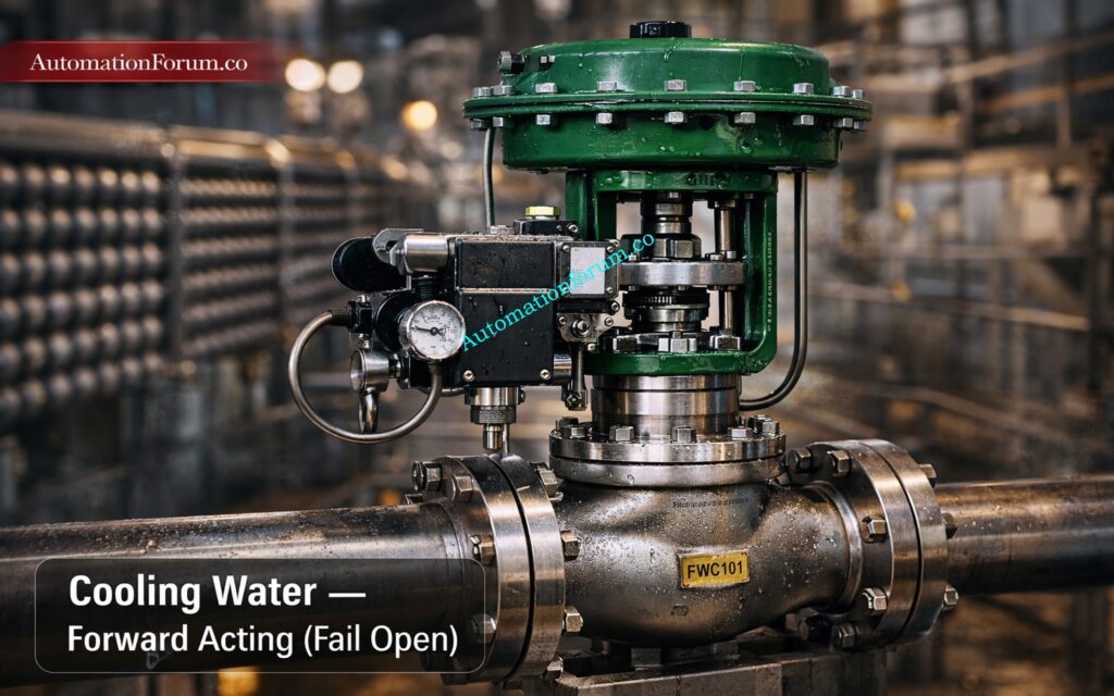
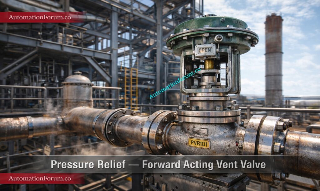
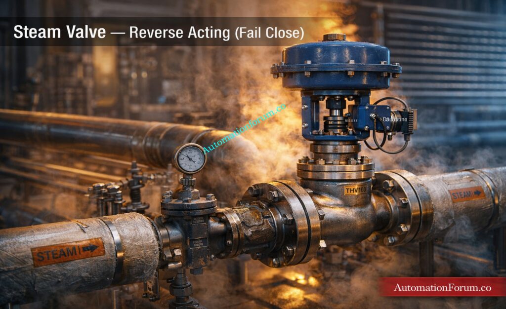
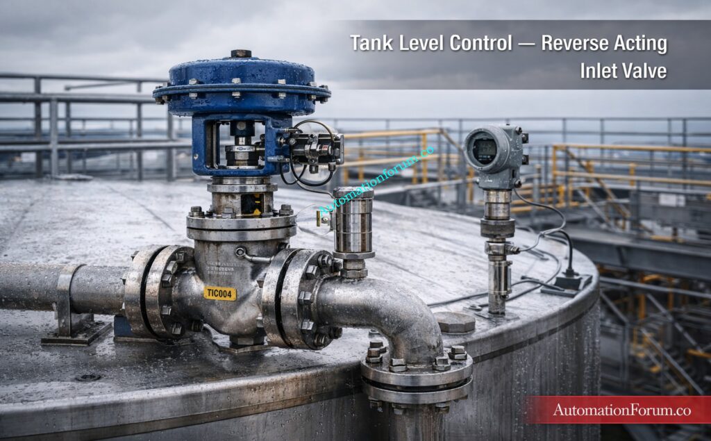

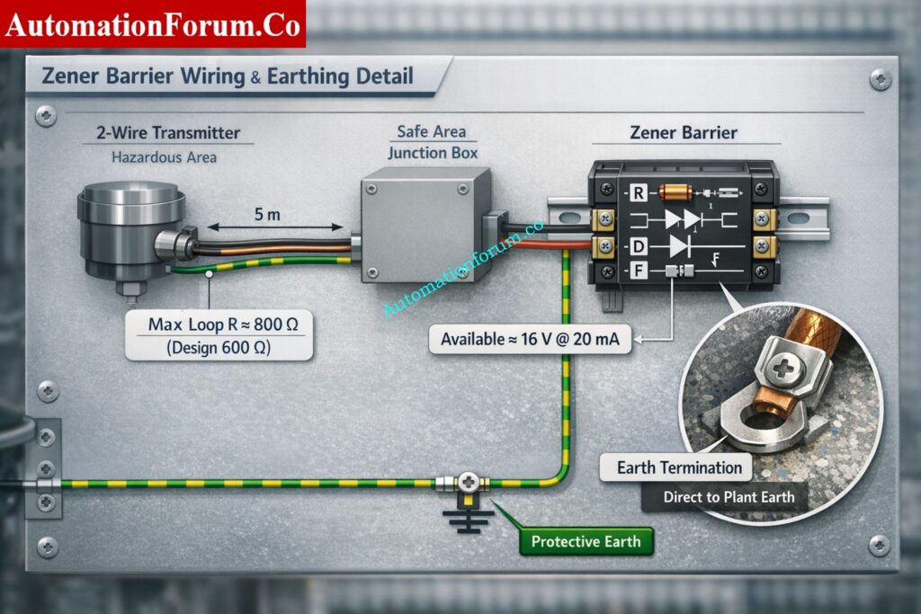
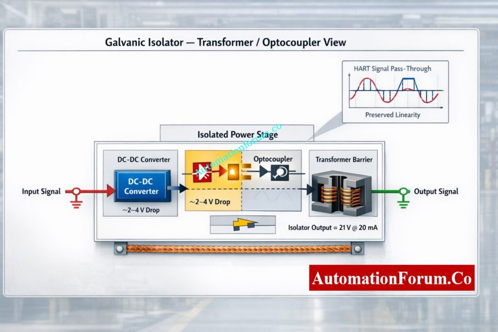
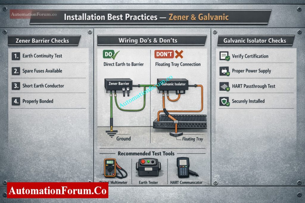
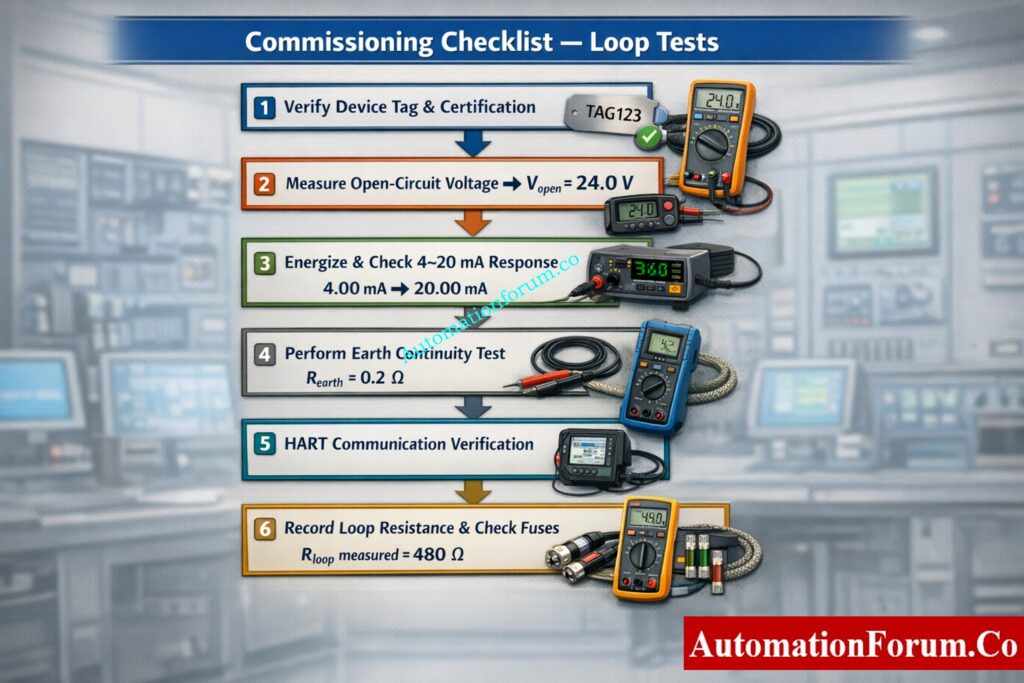
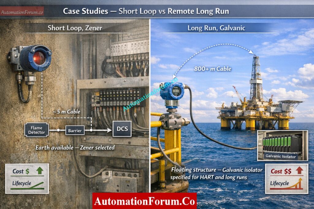

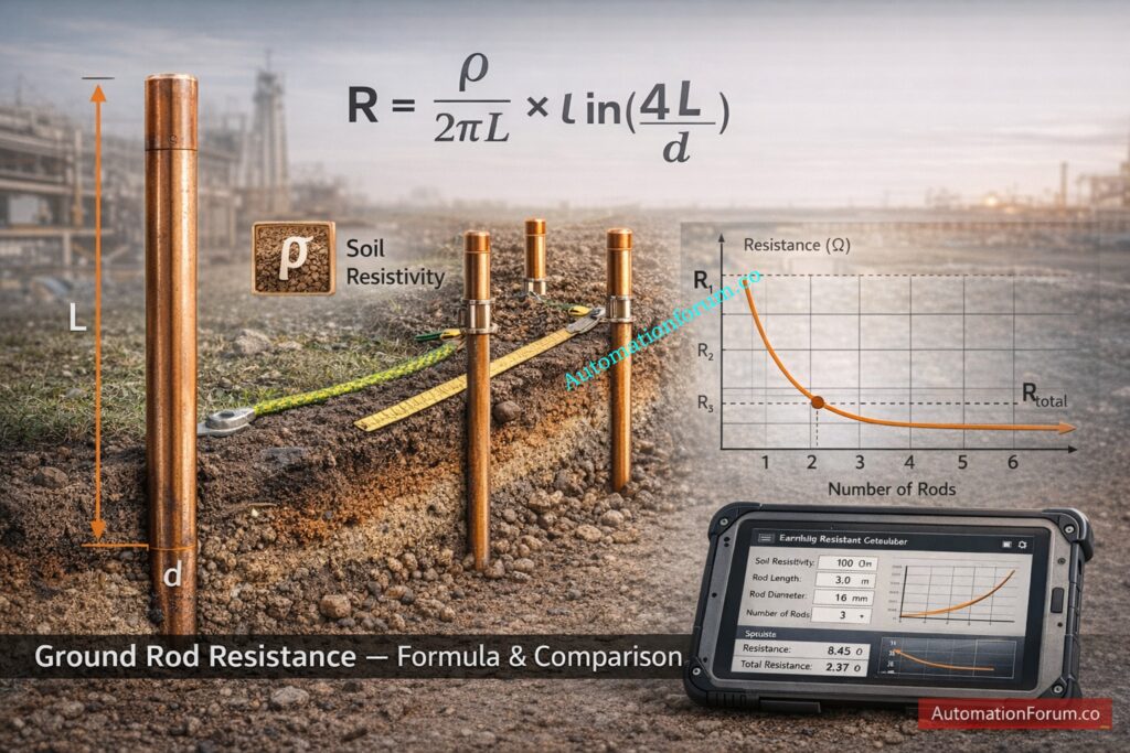

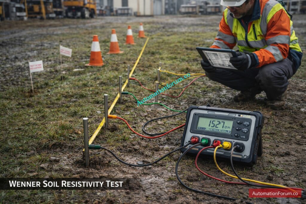

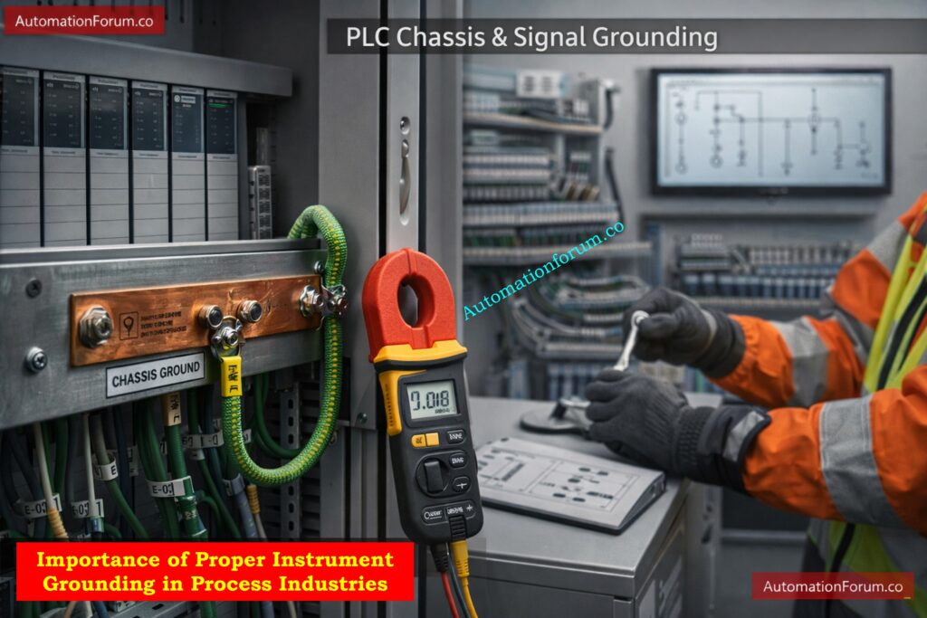

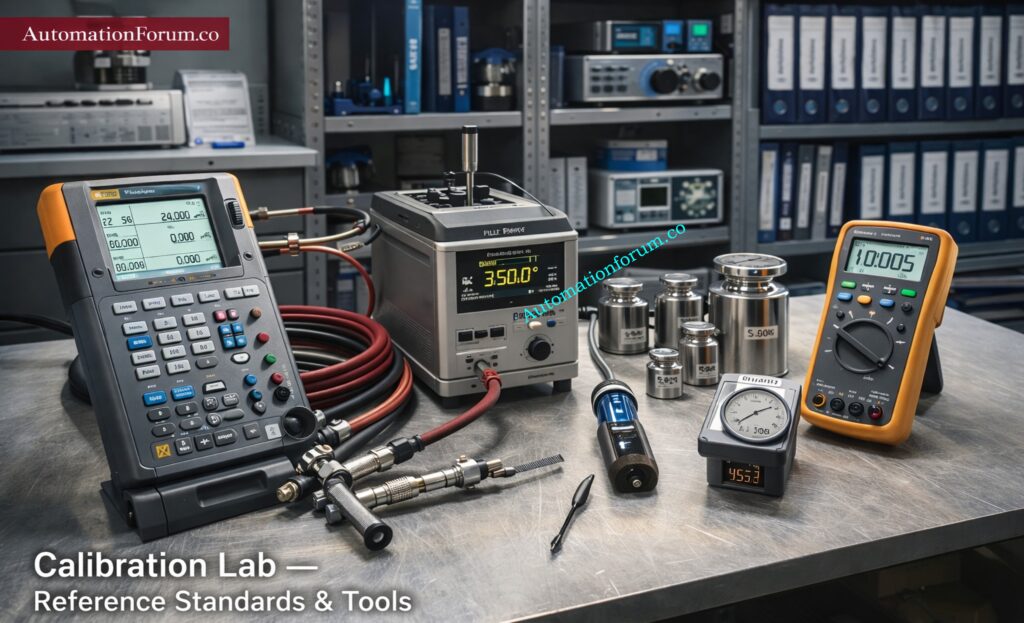
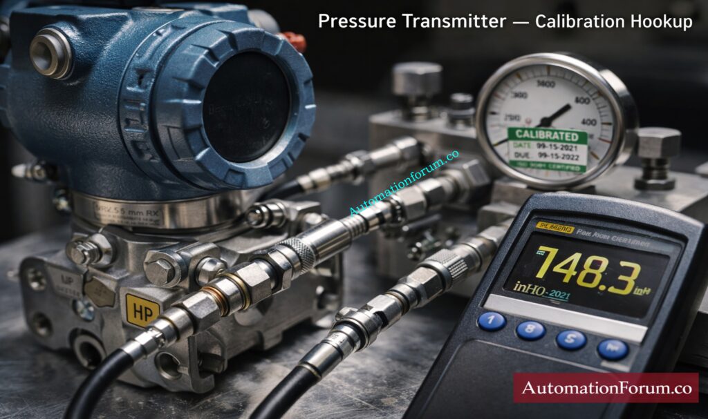
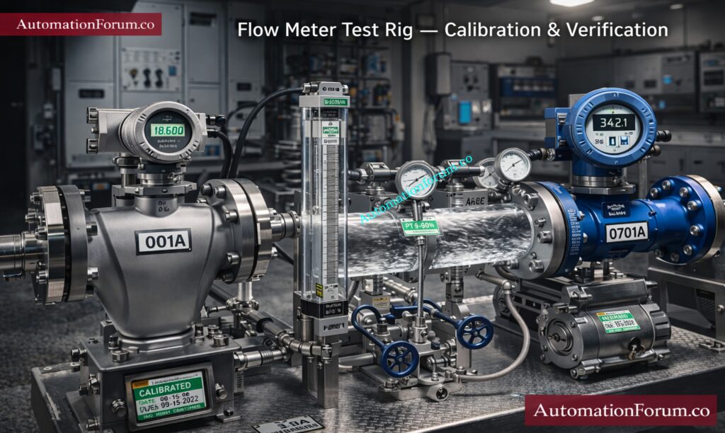
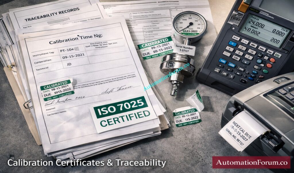
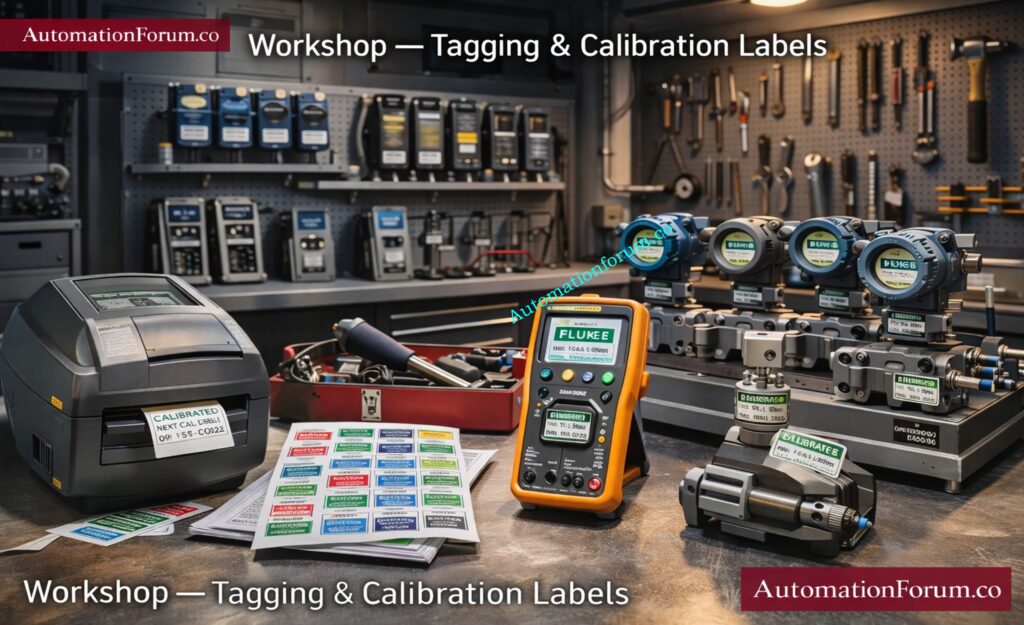
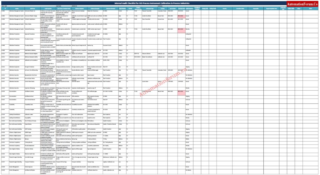


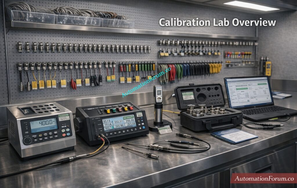
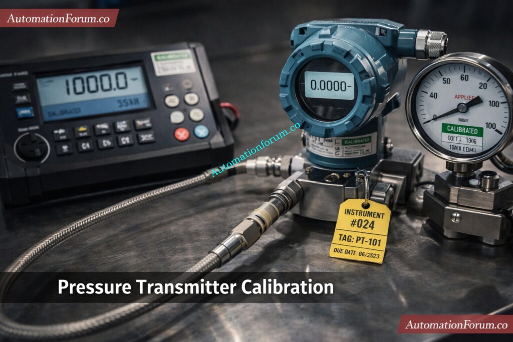
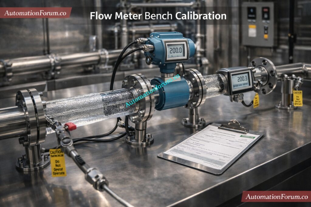
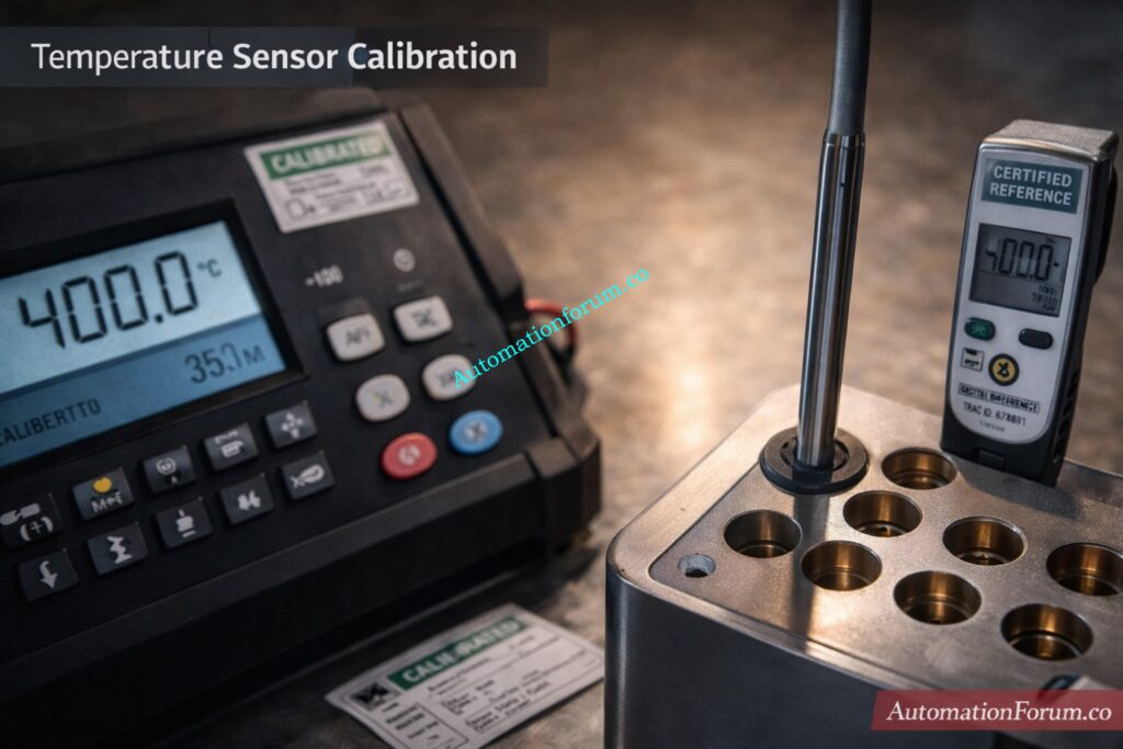
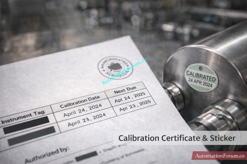
 in Industrial Automation - Complete Guide for Engineers 1")