Why Mastering PLC AO Signal Troubleshooting Matters in Process Plants
Learn how to fix PLC analog output problems with real-world, field-tested examples that focus on 4–20 mA signal problems, PLC loop problems, and instrumentation problems in the process industry. This advanced quiz focuses on finding faults in AO cards, grounding, scaling, and actuator interfaces. It gets EPC, commissioning, and maintenance engineers ready to quickly find failures under plant constraints using ladder and structured text logic interpretation and signal-path verification techniques.
Key PLC AO Faults Covered in this Scenario-Based Quiz
Twenty-five scenario-based multiple-choice questions (MCQs) test real plant AO problems and require step-by-step troubleshooting based on how PLC logic works, how signals travel from PLC AO to field devices, and how senior instrumentation engineers check things during commissioning and maintenance.
Advanced PLC Analog Output Troubleshooting Questions (25 MCQs)
Why Edge AI Based Predictive Calibration Is the Latest Trend in Instrumentation and Control Engineering
Instrumentation and control engineering has always been the backbone of safe and efficient process plant operation. Accurate measurement of pressure temperature flow level and analytical parameters directly affects product quality energy efficiency safety and regulatory compliance. For decades instrumentation professionals have relied on periodic calibration preventive maintenance and manual diagnostics to ensure reliable operation of field instruments.
However modern process plants are becoming larger more complex and more automated. Shutdown windows are shrinking and unplanned downtime is increasingly unacceptable. At the same time smart instruments generate vast amounts of diagnostic data that are often underutilized. These challenges have led to the emergence of a new trending procedure in instrumentation and control known as Edge AI based predictive calibration and instrument health monitoring.
This procedure is now being actively adopted across oil and gas chemical power pharmaceutical and fertilizer industries. It represents a major shift from time based maintenance to condition based and data driven decision making. This article explains the concept the procedure the practical implementation and the benefits in a way that is directly useful for instrumentation professionals working in process plants.
What Is Edge AI Based Predictive Instrumentation Calibration and Health Monitoring
Edge AI based predictive instrumentation is a procedure where intelligent analysis is performed close to the field instruments using edge computing devices. Instead of sending all data to centralized systems raw measurement signals and diagnostic parameters are analyzed locally using artificial intelligence and machine learning techniques.
The objective is to continuously monitor instrument health detect early signs of drift degradation or abnormal behavior and predict when calibration or maintenance is required before the instrument affects the process.
In simple terms the instrument tells you when it needs attention instead of waiting for the next scheduled calibration.
Why Traditional Instrumentation Calibration Practices are No Longer Sufficient
Limitations of Periodic Time-Based Calibration
Most process plants still follow fixed calibration intervals such as six months or one year. While this approach ensures compliance it has several weaknesses.
An instrument can drift significantly just weeks after calibration without being detected. Another instrument may remain stable for years yet still be calibrated repeatedly. This leads to unnecessary maintenance effort and cost.
Reactive Instrument Troubleshooting and Its Impact on Process Stability
Many instrument problems are discovered only after operators notice unstable readings alarms or control loop oscillations. At this stage the process is already affected and production losses may occur.
Underutilization of Smart Instrument Diagnostics in Process Plants
Modern transmitters provide valuable diagnostic information such as sensor aging impulse line plugging coating buildup and electronics health. In many plants this information is not analyzed systematically.
These gaps are precisely what predictive instrumentation procedures aim to close.
Why Edge AI Predictive Instrumentation Is Trending in Modern Process Plants
Several industry trends are driving the adoption of predictive instrumentation.
First smart instruments have become standard rather than optional. Second edge computing hardware is now affordable reliable and industrial grade. Third process industries are embracing digital transformation and asset performance management. Finally there is increasing pressure to reduce maintenance cost while improving reliability.
Major automation manufacturers such as Endress+Hauser, ABB, Siemens, Honeywell, and Yokogawa are embedding predictive diagnostics and analytics into their instrumentation and asset management platforms. This confirms that the trend is industry wide and not experimental.
Core Elements of Edge AI Based Predictive Instrumentation Systems
Smart Field Instruments and Embedded Diagnostics
The foundation of predictive instrumentation is smart field devices. These instruments provide not only the measured process variable but also internal diagnostics such as sensor signal strength noise temperature compensation and electronics health.
Examples include smart pressure transmitters flow meters radar level transmitters and analytical sensors.
Edge Computing Layer for Local Instrument Analytics
Edge devices are installed near the field or control system. They collect high resolution data from instruments and execute analytics locally. This cuts down on latency, makes things more reliable, and stops data from being sent to higher-level systems when it doesn’t need to be.
Predictive Analytics and Artificial Intelligence Models
Artificial intelligence models look at trends, patterns, and changes in how instruments behave. These models learn from past data and are always updated as situations change.
The idea is not to replace engineering judgement but to give early warnings and useful information.
Step-by-Step Edge AI Based Predictive Instrumentation Procedure
Step 1: Instrument Digital Readiness Assessment
The first thing to do is find the most important tools and see how well they work with digital technology. Instrumentation engineers should make sure that devices can communicate and diagnose problems digitally and that they are linked to an asset management system.
Instruments that affect the quality of safety products or the availability of plants should be given the most attention.
Step 2: Definition of Instrument Health Indicators
Next, engineers set measurable health indicators for each sort of device. For pressure transmitters, this might be the level of noise and the time it takes for the sensor to respond. For flow meters, it might be the strength of the signal and the balance of the sensors. For analytical instruments it may include reference deviation and calibration stability.
These indicators form the baseline for predictive analysis.
Step 3: High-Resolution Data Acquisition at the Edge
At the edge, we get high-frequency data and diagnostics. This method captures raw signal behaviour and small changes, which is different from previous systems that only look at final values.
This level of detail is necessary for early diagnosis of deterioration.
Refer the below link for the Top 10 Essential Maintenance Metrics Every Reliability Engineer Must Track
AI models always look at how things are now and how they were in the past. When the system sees strange patterns, it tries to figure out what might be causing them, such sensors being old or stress from the environment.
The system doesn’t just sound alerts; it also gives information and levels of confidence.
Step 5: Condition-Based Calibration Decision Making
Calibration doesn’t happen on a set schedule; instead, it happens when predicted indications go above certain boundaries. This makes sure that calibration is done when it is needed and not done when it is not needed.
Instrumentation teams may plan their work ahead of time instead of having to fix problems when they happen.
Step 6: Integration with Maintenance and Control Systems
The asset management system and the maintenance management system that are part of the distributed control system work together with predictive alerts. This makes a whole process from finding the problem to carrying out the work order and keeping documentation.
Practical Example: Predictive Calibration of a Pressure Transmitter in a Process Plant
Think about a differential pressure transmitter that is used to measure flow over an aperture plate in a chemical plant. This instrument directly influences flow control loop stability and process efficiency.
Traditional Calibration Approach and Its Limitations
In a conventional maintenance strategy the transmitter is calibrated every six months. Any drift caused by impulse line fouling temperature cycling or sensor aging often remains unnoticed between calibration intervals. The issue is usually identified only during routine calibration or after operators observe unstable flow readings and control loop oscillations. By this time the process may already be affected and maintenance becomes reactive.
With predictive instrumentation the transmitter continuously provides diagnostic and raw signal data to an edge analytics system. Over time the system detects a gradual increase in signal noise and a slow zero offset trend. Although the measured flow remains within limits the analytics model predicts that calibration tolerance will be exceeded within a few weeks.
Maintenance is then scheduled during normal operation or a planned low load period. The transmitter is inspected and calibrated before it impacts the process.
Operational Results and Performance Improvements
This approach improves measurement reliability stabilizes control performance reduces unplanned downtime and converts calibration from a fixed schedule activity into a condition based maintenance task.
Key Benefits of Edge AI Based Predictive Instrumentation for Engineers
Predictive monitoring makes ensuring that equipment stay within acceptable accuracy limits all the time, not only during regular calibration.
Calibration is only done when it’s needed, which cuts down on superfluous effort and lets engineers focus on more important duties related to engineering and reliability.
Early identification of instrument degradation prevents control loop oscillations nuisance alarms and unexpected process disturbances.
Condition based calibration and diagnostic records provide clear technical justification during regulatory audits quality inspections and safety reviews.
Instrumentation engineers develop valuable expertise in instrument diagnostics data interpretation and digital maintenance systems which are increasingly important in modern process plants.
Industries Actively Using Predictive Instrumentation and Condition-Based Calibration
Predictive instrumentation procedures are already being implemented in oil and gas production refineries petrochemical complexes power plants pharmaceutical manufacturing fertilizer plants and LNG facilities.
These businesses use a lot of important tools, and even tiny improvements in reliability can save them a lot of money.
Challenges in Implementing Edge AI Predictive Instrumentation and How to Overcome Them
Organizational Resistance to Condition-Based Calibration
Some teams don’t want to change their calibration schedules because they’re used to them. Pilot projects on important tools help show how useful they are.
Instrument Data Quality and Reliability Issues
Predictive systems depend on clean reliable data. Proper instrument installation grounding and shielding remain essential.
Skill Gap in Predictive Diagnostics and Analytics
Engineers do not need to become data scientists but they must understand diagnostics and trends. The most important things are training and slowly adopting.
Best Practices for Successful Adoption of Predictive Instrumentation in Process Plants
Begin with a small area of concentration on the most important tools. Set explicit standards for what makes predictive alerts acceptable. Don’t only trust algorithms; keep an eye on engineering. Don’t use predictive insights to automatically control actions; instead, use them to help you make decisions.
Future of Instrumentation Engineering with Edge AI and Predictive Maintenance
Instrumentation engineering is changing from keeping track of manual measurements to managing assets intelligently. Future instruments will be self aware capable of self diagnosis and able to communicate their health status automatically.
Engineers who embrace predictive instrumentation will play a central role in smart plant operation reliability engineering and digital transformation initiatives.
Why Edge AI Based Predictive Instrumentation Is the Future of Process Plant Reliability
Edge AI based predictive calibration and instrument health monitoring represents the most important recent advancement in instrumentation and control procedures for process plants. It addresses long standing limitations of traditional maintenance practices and unlocks the full value of smart instrumentation.
For instrumentation professionals this procedure offers improved reliability reduced workload and enhanced professional relevance in an increasingly digital industrial landscape. Using predictive instrumentation now is more than just a technological update; it’s a smart move toward the future of process automation.
FAQ on Edge AI Based Predictive Instrumentation Calibration
What is predictive calibration in instrumentation?
Predictive calibration is a condition-based method that looks at instrument performance and diagnostics all the time to figure out the best time for calibration, rather than sticking to set schedules.
How does edge AI improve instrument calibration accuracy?
Edge AI looks at raw sensor data and diagnostics on the spot, which lets it find drift, degradation, or strange behaviour early on, before measurement accuracy is damaged.
What is the difference between predictive calibration and preventive calibration?
Preventive calibration happens at set times, while predictive calibration only happens when instrument performance indicators go above certain levels, using real-time data and analytics.
Which instruments are suitable for edge AI based health monitoring?
Smart pressure transmitters, flowmeters, level transmitters, temperature sensors, and analytical instruments with digital diagnostics are all good examples of things that can be monitored with edge AI.
What data is required for predictive instrument health monitoring?
To check the health of an instrument, predictive systems look at raw sensor signals, diagnostic parameters, ambient data, historical calibration records, and operating circumstances.
How does predictive calibration reduce unplanned downtime?
Early detection of instrument problems allows for preventive repair to be scheduled before inaccurate measurements lead to control instability, alarms, or process shutdowns.
Refer the below link for the Heartbeat Technology in Process Instrumentation – Complete Working, Diagnostics, Verification & Predictive Maintenance Guide
Incident Summary: 36 Temperature Tags Dropped to Zero and Alarm Flooding
Temperature measurement is very important for safe and smooth operation in process facilities. Even a small configuration oversight can lead to large-scale disturbances. This article discusses a real incident where 18 temperature transmitters suddenly failed, eventually leading to 36 temperature tags showing zero values on the PLC, causing serious operational concern and risk of plant shutdown.
This case study shows how using the same Modbus address in temperature multiplexers caused wrong readings and how the problem was found and fixed.
Timeline & Initial Symptoms
There are eighteen temperature sensors in Area One suddenly showed 0°C on the PLC, while eighteen others in Area Two were already at zero. This caused thirty-six tags to be affected and a lot of alarms to go out in the control room. The alarm’s loudness made it hard for operators to focus, thus it had to be quickly reported to the maintenance and instrumentation teams.
Two Days Of Intermittent Zero Drops And Final Collapse
Control room operators experienced alarm overload that made it difficult to prioritize actions, and the combined loss of multiple temperature signals created immediate process safety concern and increased the probability of manual or automated trips. Restoring visibility was the top priority to keep plant systems within safe operating envelopes.
Area One showed intermittent zero drops for two days prior to the incident, with values collapsing for a few seconds and then recovering automatically, which led field teams to initially suspect transient noise grounding or sensor instability. The intermittent nature deferred higher urgency until the final sustained collapse.
The instrumentation engineer came to site under a permit to work to inspect the Area One multiplexer, confirm the fault condition, remove the suspected device, install a spare, and attempt rapid restoration of critical temperature visibility while coordinating tightly with operations.
Field Response: Safety, Permit to Work and First Actions
Permit, PPE and Control Room Historian Review
The instrumentation engineer arrived on site, obtained the permit to work, completed the safety briefing, verified PPE levels and confirmed lockout tagout points before opening enclosures or touching equipment. The permit to work sheet kept track of all planned activities.
The engineer looked at alarm lists and PLC historian trends in the control room to figure out which process variables went with which multiplexer channels and mark the timestamps. This cut down on the time spent in the field. This phase made sure that the field visit was focused on the right hardware.
At the enclosure the engineer traced instrument tags and wiring, verified terminal numbers and cross-checked drawings to avoid disconnecting unrelated circuits and to ensure safe removal of the suspected device. Wiring verification reduced risk of introducing additional faults.
Communications with operations were continuous during the activity so that any power isolation or restart was coordinated, process impact was minimized and control room operators were prepared to follow emergency procedures if unexpected consequences occurred.
Fault Led, Bench History And Why Bench Resets Are Critical
The multiplexer was powered on and showed a continuous red fault LED while measured supply voltage remained within acceptable limits, making a supply failure unlikely and pointing attention toward device internal fault or configuration anomalies.
The enclosure showed no signs of wiring damage, corrosion, or loose cable terminations. This made it less likely that the device would fail mechanically and supported a replacement plan that used a spare device to speed up recovery.
The engineer ran a controlled power cycle while the control room watched the PLC’s behaviour. The fault LED stayed on after the reboot, which confirmed that the device did not recover and that replacing it was the best way to swiftly restore measurements.
For the incident report and any vendor support or warranty return, device details including the serial number, model, and fault LED behaviour were recorded. This kept the information traceable for further study.
Spare Selection And Preinstall Checks
The engineer took a preconfigured spare multiplexer from the maintenance store and looked at the bench record, which revealed that the spare had been used on a test bench lately. This showed that the configuration needed to be checked before connecting to a live network.
Physical checks of the spare included checking the connectors, harnesses, mounting tabs, and grounding continuity to make sure the item was ready to be installed in the field and wouldn’t cause any problems with wiring or grounding.
The engineer worked with operations to set up a replacement window and made sure that the PLC would behave as expected during the removal. This way, control room staff could see trends before and after the removal and respond right away to any unexpected alarms.
The spare front panel was inspected for address and communication parameter visibility though at this stage the spare was assumed ready for field use; the subsequent diagnosis showed why explicit verification of slave ID is mandatory prior to energizing on the live bus.
Isolation, Removal, Wiring Best-Practices and Grounding Checks
The engineer isolated power at the approved isolation point, removed the faulty multiplexer while documenting the removed unit serial number and observed LED fault state, and prepared the enclosure for mounting the spare. The work order kept track of everything that happened.
The spare multiplexer was put in the same place, and the wire was re-terminated according to the designs, paying close attention to shield terminations, terminal torque, and cable routing to keep the signal clear and cut down on electromagnetic interference.
Before restoring power, the continuity of the ground between the enclosure and shield terminations was checked to make sure that the installation wouldn’t add noise to the measurement loops.
Power was restored to the spare while the engineer notified the control room to watch PLC process values and alarms in real time so any new anomalies could be correlated with the exact instant of energizing the spare.
Timestamps And Correlation That Pointed To A Network Conflict
Within seconds after turning on the spare, a different set of eighteen temperature tags in Area Two dropped to zero on the PLC. However, the Area Two multiplexer displayed healthy LEDs and a consistent supply, which meant that the problem was not a local hardware failure in Area Two.
The control room and field crew looked at the timestamps of the events and saw that the values in Area Two matched the time when the spare was turned on in Area One. This clearly suggests that there was a network-level conflict rather than two devices failing at the same time.
The engineer worked with operations to set up a controlled isolation test. They turned off the Area Two multiplexer for a short time while keeping an eye on the PLC to see what data was still on the bus and how mapping changed when devices were taken away.
When the Area Two multiplexer was turned off, the values came back, but the tags showed temperatures from Area One. This was the key indicator that two devices were sending data to the same Modbus address, which messed up the PLC mapping logic.
When Area Two was turned off, the mapping of Area One values into Area Two tags showed that two devices were responding to the same Modbus address. This meant that the PLC couldn’t tell which device sent which data, which led to the wrong assignment.
The engineer looked at the spare multiplexer front panel and checked the communication settings. This confirmed that the slave ID had been modified during bench testing and had not been reset to a unique spare address before installation.
We connected a handheld Modbus scanner to the RS485 bus and used it to check for expected slave IDs. The scanner data showed overlapping responses and frame durations that didn’t match up, which meant that more than one device was responding to the same address.
We looked at the PLC communication diagnostics and saw that there were more CRC failures, timeouts, and retry counts during the conflict. These diagnostics backed up the scanner information and supported the idea that the duplicate address was the reason.
Root Cause Identification: How Duplicate Ids Corrupt PLC Mapping And Create Crc Errors
The spare multiplexer retained a test bench Modbus slave ID that matched the Modbus ID of the Area Two multiplexer, resulting in duplicate slave addresses on the same RS485 bus.
Two devices attempting to answer the same PLC query produced overlapping response frames corrupted data and CRC errors which the PLC driver rejected or interpreted incorrectly leading to zero or default values being presented to operators.
When one device was removed or powered down the PLC read from the remaining device but mapped the registers based on expected index and sequence, which caused values to appear under incorrect tags until addresses were made unique.
The core failure drivers were human and process gaps in bench reset procedures and absence of a mandatory preinstall address verification step that would have prevented placing a bench configured spare on the live network.
Change Slave Id, Verify With Modbus Scanner, Live Signal Verification
The engineer changed the spare multiplexer Modbus slave ID to a unique free address using the device front panel, confirmed the new address with the handheld Modbus scanner and verified the device responded singularly at that address.
Area Two multiplexer was powered back on and the PLC communication diagnostics were observed to confirm CRC errors and timeout counters ceased increasing and normal request response timing resumed.
Live signal verification was performed for each restored tag: the engineer measured field temperature with a calibrated handheld instrument compared those values to the PLC process variables and recorded the results for every channel to confirm correct mapping and sensor performance.
Records were updated: the central Modbus address register was modified to include the new assignment device serial number and change date, CMMS work order was completed with attachments and the newly configured devices were labeled with durable address plates.
Mandatory preinstall Modbus address check and centralized register
Measure field temperature at transmitter TMP101 using a calibrated thermometer and record 145 degrees Celsius, confirm PLC PV TMP101 reads 145 degrees Celsius at 10 32 and sign verification sheet with technician name and date.
Repeat the same measurement and comparison for TMP102 through TMP118 recording each field value PLC PV mapping status and noting any discrepancies along with corrective actions taken.
Monitor each restored tag for a stability period of five minutes and confirm three consecutive consistent readings before final sign off; log any communication retries or CRC events observed during verification for follow up.
Add screenshots of the PLC trends taken before the removal and after the restoration to the work order. Also, include pictures of the front panel of the device showing the new Modbus ID and the label that was put on it for audit purposes.
PLC Remote I/O Card Failure Can Trip the Entire Plant: Root Cause Analysis of PLC Remote I/O Panel (Point I/O Panel) Cards Failure Issues (Refer below link)
Before racking out any field device, get a work permit, double-check the isolation points, and write down the spare serial number in the work order.
Verify spare Modbus slave ID against the centralized Modbus address register and set the spare to the approved spare ID if necessary before connecting to the live bus.
If the spare was utilised on a test bench, reset it to the approved spare address, write down the time and date of the bench log entry, and attach the log to the spare record.
Work with the control room to set up a controlled replacement window. Keep an eye on the PLC trend buffers the whole while the replacement is happening, and take pictures before and after the replacement for incident analysis.
Practical Modbus Scanner and PLC Diagnostics Steps
Connect the Modbus scanner to the RS485 pair and the common ground. Set the scanner to match the network parameters, such as baud rate, parity, and stop bits. Then, poll the slave IDs one at a time to find unexpected replies.
Check the scanner output for frames that overlap, frame lengths that don’t match, or repeated responses. Then, export the logs you captured to add to the maintenance record and incident report.
Check the PLCcommunication diagnostics for things like CRC error counts, timeout occurrences, retry counters, and request response latency. You may use timestamps to link these metrics to scanner captures and events in the control room.
If you keep getting the same answers after readdressing capture sample frames serial numbers, you should contact a control systems specialist or vendor support with the proof you have.
Preventive Controls and Process Changes to Implement
Add required Modbus address verification to checklists for replacement and commissioning, and make sure that no spare is linked to the active bus until it has been signed off on. This step must be included in the permit to work closure criteria.
Maintain a central Modbus address register that includes device tag serial number model assigned address physical location and last updated date and make it accessible to operations maintenance and instrumentation teams.
Label every addressable device on the front plate inside the enclosure and on the enclosure door showing Modbus ID device tag and last configuration date so field crews can visually confirm settings before installation.
Set up a bench configuration log system that makes bench engineers write down any temporary address changes and put devices back to an approved spare address before putting them back in inventory. This should be checked by a supervisor.
Only authorised instrumentation workers should be able to alter Modbus addresses, and a logged change history should be kept that shows the rationale, approver, and timestamp of each change to stop unauthorised or undocumented changes.
Add spare device fields to the CMMS with the spare serial configuration status, the date of the next verification, and reminder alerts so that spares are checked before they are used.
Do audits every three months to check that the entries in the physical labels register and the CMMS records match up, and fix any problems within a set SLA to keep the register’s integrity.
Include the incident scenario and reaction actions in regular toolbox discussions and shift handovers so that technicians and operators know what to look for when they see duplicate addresses and implement the isolation procedure right away.
Pre replacement verification: verify spare device serial number confirm bench configuration status and Modbus ID against master register, affix a verified address label to the spare and record verification details in the work order.
Replacement step: under permit to work isolate multiplexer power remove faulty device install spare re-terminate wiring and verify shielding and grounding before restoring power while operations monitors PLC trends.
Post replacement verification: perform live signal verification for each restored tag, update the Modbus address register and CMMS, attach trend screenshots and device photos to the work order and close the permit with signatures.
Refer the below link for HART Transmitter Diagnostics: What Your Field Device is Telling You
KPI And Monitoring Suggestions After Implementation
Track mean time to restore for duplicate address incidents and measure the time from alarm escalation to full restoration and verification, with a goal to reduce this interval through process controls and training.
Keep an eye on how well spare verification procedures are being followed and set a goal percentage of spares that are checked before installation. If they aren’t followed, report it so that remedial action can be taken.
Check the completion rate and resolution time for quarterly Modbus register audits, and try to fix any inconsistencies within the agreed-upon SLA periods.
Check the trends in communication problems every month and connect problems that happen more than once to the end of remedial action to make sure that things keep getting better.
At 09 15 operations reported intermittent zero values on eighteen Area One temperature tags. The instrumentation engineer attended site obtained permit to work inspected the multiplexer observed a persistent red fault indicator and removed the unit for replacement.
At 10 05 the spare multiplexer was installed. Immediately after energizing Area Two tags collapsed to zero. Coordinated isolation revealed duplicate Modbus address on the spare retained from bench testing. Spare ID was changed to a unique address and normal readings were restored. All thirty six tags were verified against field instruments within tolerance and records were updated in CMMS and the Modbus register.
Treat Modbus address verification as a mandatory preinstall check for any spare device or replacement, and record the verification in the work order to ensure accountability.
A brief verification step and a durable label on each addressable device will prevent hours of troubleshooting lost production and unnecessary operational risk.
Incorporate the SOP paragraphs live verification templates and the incident narrative into training and commissioning materials so the whole team recognizes the symptom pattern and follows the correct isolation and verification steps.
Frequently Asked Questions On Duplicate Modbus Address Issues
What is illegal data address error in Modbus?
An illegal data address error occurs when the Modbus master requests a register or coil that does not exist in the slave device. The slave responds with an exception indicating the requested address is outside its supported memory range.
What is the addressing mode of Modbus?
Modbus uses a master–slave (client–server) addressing mode where each slave device has a unique address. The master communicates by sending requests to a specific slave address on the network.
What are the weaknesses of Modbus?
Modbus has no built-in security, authentication, or encryption, making it vulnerable to unauthorized access. It also relies on polling, which can limit performance and scalability in large or fast control systems.
What is the standard addressing for Modbus?
Modbus uses logical data areas such as coils, discrete inputs, input registers, and holding registers. Internally, addressing starts from zero, even though documentation often shows addresses starting from one.
How to configure Modbus address?
A Modbus device address is configured using hardware switches, a front-panel menu, or configuration software. The address must be unique on the network to prevent communication conflicts and data corruption.
What is the maximum device address in Modbus?
In Modbus RTU and ASCII, valid slave addresses range from 1 to 247. Address 0 is reserved for broadcast messages and cannot be used for individual device communication.
The MIMO Decoupling Matrix Designer is a steady state analytical calculator used in instrumentation,automation, and process control engineering to analyze and reduce interaction between multiple control loops. In many industrial processes, a single manipulated variable affects more than one controlled variable. Likewise, each controlled variable may be influenced by multiple manipulated variables. This multivariable interaction makes conventional PID loop tuning difficult and often results in oscillations, slow response, and unstable control behavior.
The MIMO Decoupling Matrix Designer provides engineers with a structured and mathematical way to understand these interactions before implementing or modifying control strategies. By using steady state process gain data, the calculator supports correct loop pairing decisions, evaluates whether decoupling is feasible, and generates a decoupling matrix that can be used to reduce loop interaction. The tool is especially valuable during control system design, commissioning, and troubleshooting.
What Is a MIMO Decoupling Matrix Designer in Process Control
Definition of MIMO Decoupling Matrix Designer
The MIMO Decoupling Matrix Designer is a steady state multivariable control analysis tool based on the process gain matrix. Each element of the matrix represents the steady state influence of a manipulated variable on a controlled variable. The calculator uses math to figure out how strongly control loops interact with each other and if static decoupling can help lessen those interactions.
This calculator just looks at steady state behaviour and doesn’t take into account things like dead time, temporal constants, or nonlinear reactions. Instead, it provides fast and reliable insight into whether decentralized control is reasonable or whether more advanced control strategies such as model predictive control are required.
Meaning of MIMO in Industrial Automation Systems
Engineers in real-world industrial settings frequently encounter stringent deadlines and restricted availability of sophisticated modelling tools. The MIMO Decoupling Matrix Designer fills this gap by allowing rapid analysis using step test data or linearized process models. It acts as a bridge between basic PID control and advanced multivariable control design.
Purpose of the MIMO Decoupling Matrix Designer Calculator
Evaluating Steady State Interaction Between Control Loops
The main job of the calculator is to figure out how much control loops interact with each other when they are in steady state. Engineers can utilise numbers to figure out which controlled variable should regulate which process variable instead of depending on expertise or trial and error. This lowers the chance of bad loop pairing and makes control work better overall.
Selecting Proper Manipulated Variable and Controlled Variable Pairing
The calculator generates a decoupling matrix by inverting the process gain matrix. When used correctly, this decoupling matrix takes into account steady state interactions such that each controller output only affects the controlled variable it was meant to. This improves loop independence and simplifies PID tuning.
Determining Feasibility of Static Decoupling
The tool evaluates the condition number and determinant of the process gain matrix. These indicators reveal whether matrix inversion is safe or whether the system is numerically sensitive. This stops engineers from using decouplers that could make noise, modelling mistakes, or other problems worse.
Who Should Use the MIMO Decoupling Matrix Designer
Control and Instrumentation Engineers
During design and commissioning, control and instrumentation engineers utilise the calculator to explain why they paired up control loops. It helps them make written and defensible control plans for the teams that run and maintain things.
Advanced Process Control Engineers
Before spending time on dynamic modelling or constructing model predictive control solutions, advanced process control engineers use the calculator as a screening tool. It helps identify whether simple decoupling is sufficient or whether full multivariable control is required.
Commissioning and Startup Teams
Commissioning teams use the calculator on site after performing step tests. It allows them to confirm that the selected manipulated variable to controlled variable mapping behaves correctly at the operating point.
Maintenance and Production Support Teams
When process modifications or equipment aging introduce unexpected interaction, maintenance and production support teams use the calculator to identify whether the root cause is steady state coupling, instrumentation issues, or control configuration errors.
Industrial Applications of MIMO Decoupling Matrix Designer
Industrial Applications
The calculator is widely used in oil and gas refineries, petrochemical plants, chemical processing units, power plants, water treatment facilities, and pharmaceutical manufacturing. These industries commonly operate processes with strong multivariable interactions, such as distillation columns, reactors, boilers, and pump networks.
Control System Lifecycle Stages
The calculator is applied during early control architecture design, commissioning, control optimization projects, and troubleshooting activities. It is equally useful in greenfield projects and brownfield upgrades.
Control Philosophy and Functional Design Specification
The control philosophy paper and the reports on loop interaction studies should have the calculator linked to it. Placing the calculator results alongside the control narrative allows reviewers and auditors to understand the technical basis of loop pairing and decoupling decisions.
Loop Tuning and Commissioning Records
During commissioning, the calculator should be included as part of the loop commissioning dossier. This includes the raw step test data, the process gain matrix, the decoupling matrix, the relative gain array, and numerical stability indicators. This documentation becomes valuable during future troubleshooting and audits.
Engineering Calculation Repositories
For EPC projects and system integrators, the calculator is best attached to the engineering calculation repository or instrument index system. This ensures that future modifications use the same analytical foundation rather than repeating trial-and-error tuning.
PLC and DCS Configuration Documentation
When you use decoupling in PLC or DCS logic, you should write down the calculator output in the control configuration notes. This ensures that future engineers understand why the decoupling logic exists and under what conditions it is valid.
The process gain matrix is constructed by applying small step changes to each manipulated variable and observing the steady state change in each controlled variable. These gains form the mathematical foundation of the calculator.
Steady State Gain Identification Using Step Testing
If the process gain matrix is invertible and numerically stable, the inverse matrix becomes the decoupling matrix. This matrix is used to make up for the steady state interaction between loops.
Decoupling Matrix Calculation Using Matrix Inversion
The calculator uses the relative gain array to figure out how good the pairing is. Values close to one mean that the pairings are good, while negative or very high values mean that the loop assignments could be unstable or not what you want.
Relative Gain Array Calculation and Interpretation
The calculator uses the condition number and determinant to check how stable numbers are. Engineers use these numbers to figure out if static decoupling is safe or if they need to use different methods.
Limitations of the MIMO Decoupling Matrix Designer
Steady State Only Modeling Limitations
The calculator doesn’t take into consideration things like dead time or process slowness that change with time. Final validation still needs dynamic analysis and simulation.
Effect of Nonlinear Process Behavior
The tool assumes linear behavior around an operating point. Highly nonlinear processes require repeated analysis at multiple operating conditions or gain scheduling.
Sensitivity to Measurement Errors and Instrument Accuracy
The accuracy of the calculator depends entirely on the quality of steady state gain data. Poor step tests or noisy measurements lead to unreliable results.
In practical industrial applications, the process gain matrix may be poorly conditioned or nearly singular due to measurement noise, weak coupling paths, or insufficient excitation during step testing. In some situations, direct matrix inversion might create decoupling improvements that are too big, which makes noise and disturbances worse.
So, before inverting, the MIMO Decoupling Matrix Designer checks for numerical robustness. Engineers should not use direct inversion if the determinant of the process gain matrix is near to zero or the condition number is too high. Instead, you can use other numerical methods like the Moore–Penrose pseudo inverse or regularised inversion.
Regularisation adds a modest stabilising term that makes the structure of the main interaction less sensitive to noise. This stops the controller’s output from being amplified too much and makes it easier to use in PLC or DCS settings.
Input Data Requirements for Accurate MIMO Decoupling Analysis
The MIMO Decoupling Matrix Designer’s correctness is highly contingent upon the quality of the steady state gain data utilised in the construction of the process gain matrix. When you change one variable, you should just change that variable and leave all the others the same. The step size needs to be big enough to get rid of measurement noise but small enough to keep the behaviour around the operational point linear.
You can only record steady state values after the controlled variables have completely settled. Using transient readings or not fully settling can provide wrong gain estimates and misleading decoupling results. To lessen the effect of noise, it is best to average the final steady values across a sufficient time span.
You must use the same engineering units or normalised units for all gains. If you don’t scale the units correctly, the relative interaction strength can be wrong, and the relative gain array values can be wrong too.
Before using the decoupling matrix in a control system, it needs to be checked for accuracy. One important step in checking is to multiply the decoupling matrix by the original process gain matrix. The ideal outcome is that the product should be close to an identity matrix, which shows that steady state decoupling is working well.
Any significant divergence from the identity matrix signifies numerical instability, inadequate data quality, or excessive interaction that cannot be mitigated with static decoupling. In these circumstances, engineers should go over gain data, perform step tests, or think about other ways to control things.
All process gain values used in the MIMO Decoupling Matrix Designer are affected by transmitter accuracy, resolution, and noise. Small mistakes in estimating gain can spread through matrix inversion and have a big effect on how well decoupling works.
Engineers should look at realistic gain adjustments and see how much the decoupling matrix changes to figure out how sensitive it is. Highly sensitive systems suggest that static decoupling may lack the durability required for prolonged operation, especially in the context of process variability or equipment ageing.
Implementation Considerations in PLC and DCS Systems
Decoupling Logic Placement in Control Architecture
When implementing the decoupling matrix in a PLC or DCS, careful attention must be given to signal scaling and limits. The decoupling logic modifies controller outputs before they reach the final control elements. If actuator limits are reached, interaction compensation may become incomplete or asymmetric.
Anti Windup Strategy for Decoupled PID Controllers
Anti windup mechanisms must be enabled in individual PID controllers to prevent integrator saturation caused by decoupling corrections. Signal conditioning and filtering should also be evaluated to avoid amplifying measurement noise through the decoupling matrix.
Clear documentation must be added to control logic descriptions explaining why decoupling is used, the operating range for which it is valid, and any assumptions made during design.
Processes With Dominant Dead Time & Strongly Varying Operating Conditions
The MIMO Decoupling Matrix Designer is intended for steady state interaction reduction only. It is not suitable when process dynamics differ significantly between loops, when dead times are dominant, or when interactions vary strongly with operating conditions.
Cases Requiring Advanced Multivariable Control
If loop dynamics are highly dissimilar or if interaction changes with throughput, temperature, or composition, static decoupling may degrade dynamic performance. In such situations, engineers should consider dynamic decoupling or advanced multivariable control techniques.
The MIMO Decoupling Matrix Designer is a useful and sophisticated engineering tool that gives you important steady state information on multivariable control problems. When used appropriately and documented accurately, it helps make better decisions about loop pairing, safer decoupling, and speedier debugging. Attaching the calculator to control documents, commissioning records, and engineering knowledge bases makes sure that the control system will be used for a long time and that it will work the same way throughout its existence.
A decoupling matrix is a math matrix used in multivariable control systems to make sure that control loops don’t interact with each other as much.
It comes from the inverse of the process gain matrix and makes up for steady state cross coupling. Decoupling matrices help each manipulated variable primarily affect its intended controlled variable.
What is the concept of MIMO?
MIMO stands for “multiple input multiple output.” It describes systems that have more than one input that can be controlled and more than one output that can be controlled.
In MIMO systems, each input can affect more than one output, which causes loops to interact with one other.
Mutual coupling in a MIMO antenna occurs when electromagnetic energy from one antenna element affects nearby elements. This interaction changes antenna impedance, radiation patterns, and signal correlation. Reducing mutual coupling improves MIMO system capacity, efficiency, and signal quality.
What is the CCL in MIMO?
CCL in MIMO refers to Channel Capacity Loss caused by correlation and mutual coupling between antenna elements. It represents the reduction in achievable data rate compared to an ideal uncorrelated MIMO system. Lower CCL values indicate better MIMO antenna performance and higher communication reliability.
What does 3×3 MIMO mean?
3×3 MIMO means a system with three transmitting antennas and three receiving antennas. It allows up to three parallel data streams to be transmitted simultaneously. This configuration improves data throughput, reliability, and spectral efficiency compared to single-antenna systems.
This Standard Operating Procedure describes a complete and practical method for live signal verification of 4 to 20 mA analog loops used in industrial process plants. It is written specifically for instrumentation technicians commissioning engineers and maintenance professionals who work with transmitters control systems and field wiring. The procedure’s main goal is to check the health of signals in real-world situations and find faults that static calibration can’t find.
Purpose: Live Signal Verification for 4-20 mA Loops
Live signal verification ensures that a 4 to 20 mA loop performs correctly while the process is running. Unlike bench calibration or isolated loop checks live verification evaluates the entire signal path including the transmitter wiring marshalling panels barriers isolators input cards and control system scaling.
This process helps find problems with grounding and shielding, electrical noise interference, wrong barrier behaviour, and input cards. It also makes sure that the real field current is the same as the DCS or PLC process value that is shown. Live verification is critical during commissioning after maintenance and during troubleshooting of unstable or drifting signals.
This SOP applies to all conventional analog 4 to 20 mA loops including two wire three wire and four wire transmitters. It covers pressure temperature flow level and analytical transmitters connected to PLC or DCS analog inputs.
The procedure applies to operating plants utilities packaged equipment and EPC project commissioning. Safety instrumented system loops are excluded unless formal authorization and bypass approval are obtained. The procedure does not replace calibration but complements it by validating real world performance.
Electrical Safety & Personal Protective Equipment (PPE)
Before starting any live signal verification activity ensure compliance with site electrical safety rules. Wear flame resistant clothing safety shoes helmet eye protection and electrical rated gloves where required. Only use instruments that are insulated and test leads that have been approved. Stay away from open terminals with your hands to avoid short circuits.
Permit to Work & Operations Coordination
If plant procedures say you need one, get a permit to work. Before you touch any live loop, let the control room and operations staff know. Make it clear what the job will entail, particularly whether a simulation or temporary loop opening is intended. Record the name of the operations representative and approval reference.
Lockout-Tagout (LOTO) & Live Work Boundaries
Live signal verification normally does not require lockout tagout since the loop remains energized. If the loop must be disconnected for series measurement or simulation follow the lockout tagout procedure strictly. Never break a loop controlling an active process without operations approval.
Safety Instrumented System (SIS) Restrictions
Do not perform live signal verification on safety instrumented system or emergency shutdown loops unless written authorization is issued. The loop must be bypassed according to site procedures and a safety representative must be present. All SIS related work must follow functional safety rules.
Refer the below link for Why 4-20 mA Current Signal is Preferred Over Voltage Signal in Instrumentation?
Use calibrated instruments suitable for industrial environments. Commonly used tools include a digital multimeter with DC milliamp measurement capability a hand held loop calibrator that can measure and source current a HART communicator for digital diagnostics and a DC clamp meter capable of measuring low current accurately.
Clamp meters are preferred for non intrusive checks. Loop calibrators are required for simulation and linearity testing. All instruments must have valid calibration certificates.
Hand Tools & Site Accessories
Use insulated screwdrivers torque controlled terminal drivers fused test leads insulated crocodile clips and approved intrinsically safe accessories in hazardous areas. Carry a flashlight for cabinet inspection and clean cloths for removing dust or moisture.
Documentation Required at Site (Datasheets, Loop Drawings, I/O List)
Always carry the instrument datasheet loop wiring diagram hook up drawing I O list and loop index. Review previous calibration and verification records before starting work. These papers assist figure out what values are expected and what problems have happened in the past.
Pre-Verification Checks Before Measuring Loop Current
Tag Number & Loop Identification
Check the transmitter tag number in person at the field equipment. Check that it matches the wiring diagram’s loop number and the DCS or PLC tag name. Make sure you’re working on the right loop by checking the terminal numbers on the marshalling panel and the channel assignments on the input card.
Datasheet and Range (LRV/URV) Confirmation
Check the instrument datasheet to make sure the lower range value and upper range value are set correctly. Check that the output signal is 4 to 20 mA and not something else. Make sure that the engineering units and scaling in the control system are the same as those in the transmitter setup.
Visual Inspection of Installation
Inspect the transmitter junction box cable glands and conduit for mechanical damage corrosion loose fittings or moisture ingress. Check that terminal screws are tight and that the cable shield is terminated according to site grounding philosophy. Inspect barriers or isolators for fault indicators or abnormal status lights.
If any physical defect is found correct it before proceeding with live verification.
Live Signal Verification Procedure in Operating Plant
Preparation and Initial Observation
Notify Control Room and Operations Team
Confirm permit-to-work (if required) and note permit ID.
Tell the control room the exact start time, estimated duration, and whether you may briefly open the loop or simulate the signal.
Record the name and contact of the operations representative who acknowledged the work.
PPE, Safe Access and Test Equipment Readiness
Put on site-specified PPE (FR clothing, safety shoes, helmet, eye protection, electrical gloves if required).
Make sure that equipment and test leads are insulated and, if necessary, safe to use.
Verify safe access to the transmitter and marshalling panels (clear walkways, no wet surfaces).
Confirm device identity and paperwork at the device
Physically read the transmitter tag and serial number at the device and confirm it matches the loop drawing, I/O list and DCS tag.
Open the loop folder or pull up datasheet, LRV/URV, wiring diagram, marshalling layout and previous verification/calibration record. Note last calibration date.
Baseline DCS/PLC Trend Observation
Pull up the live trend for the tag and observe for at least 3–5 minutes (longer if signal is known to be intermittent).
Take a screenshot or print the trend and note the start and end times of the observation.
Record the PV, engineering units, any alarms that are going off, and the input quality/status bits that the DCS/PLC shows.
Record Ambient Conditions and Process Context
If there are any corrosive or unclean circumstances, be sure to note the temperature, humidity, and other factors.
Record process state (steady, ramping, batch cycle, startup/shutdown) and any nearby activities (motor/ compressor starts, valve cycles) that might influence noise.
Prepare Measurement Log and Verification Records
Create or open the verification log with fields: tag, location, LRV/URV, expected PV, start time, technician, operations contact.
Verify test equipment calibration sticker/date, set clamp/meter to correct DC mA range, and check meter leads and fuses.
Isolate only the terminal cover; do not remove or disturb other wiring unnecessarily.
Verify which conductors are the signal positive, signal negative, and where the cable shield is terminated. Photograph the terminal layout if helpful.
Preferred Non-Intrusive Measurement Using DC Clamp Meter
Set the clamp meter to DC mA mode (or µA if required). Confirm the clamp can measure DC current for the loop range.
Separate or spread the conductors so the clamp surrounds only the single positive signal conductor clamping both conductors will read near zero.
Place the clamp on the positive conductor only, wait for the reading to stabilise, then record: measured mA, time, meter model/ID, and meter calibration date.
Note any visible cable damage, loose terminals, or corrosion while the cover is off.
Alternative Inline (Series) Measurement with Operations Approval
Obtain clear, written or radio approval from operations to briefly open the loop. Confirm consequences to process control.
Switch meter to mA series measurement, verify correct jack/fuse installed, and brief operations that the loop will be open for a few seconds.
Loosen the positive terminal, insert the meter in series (positive wire → meter → terminal), take the reading quickly, then fully restore the connection and torque to spec.
Immediately confirm DCS behavior and that no alarms were triggered by the brief interruption. Log duration of open loop and who approved it.
Measurement Recording and Time Synchronization
Always timestamp each measurement and record the exact meter/clamp settings.
If multiple readings are taken, average or list each sample with its timestamp.
Note any discrepancy between successive readings, intermittent jumps, or unstable readings.
Safety Notes and Common Measurement Pitfalls
Never short loop wires with test leads; avoid inserting scope ground clips across loop conductors.
If the conductors are in a tight shielded cable and cannot be individually clamped, do not force separation – use the series method only if approved.
If you see near-zero current unexpectedly, stop and re-check wiring and DCS status before proceeding.
Simultaneous Field Current and DCS/PLC PV Observation
While measuring field current, have an operations person or colleague read and record the DCS/PLC PV and input quality flag at the same instant (synchronise timestamps).
If you cannot observe both simultaneously, take time-stamped meter readings and immediately capture the DCS PV screenshot with the same timestamp.
Conversion of Measured mA to Engineering Units
Convert measured mA to %span: %Span = (mA − 4) / 16 × 100.
Convert %span to PV: PV = LRV + (%Span/100) × (URV − LRV). Record calculated PV and compare to DCS PV.
Compute Δ (difference) and Δ as % of span; record whether it is within site tolerance.
Input Quality Status and Alarm Verification
Record any input quality bits (good, bad, stale, overflow, underflow) and any alarm or diagnostic messages.
If DCS shows bad/stale but field mA is valid, suspect wiring, marshalling, or input card fault – note immediately for troubleshooting.
Dynamic Response and Signal Latency Assessment
If process PV is changing, keep track of how long it takes for the DCS to update after the measured mA changes. For reference, write down the scan time or estimated delay.
If there is any lag, sluggishness, or step changes in DCS PV that don’t match changes in measured current, write them down.
Deviation Analysis and Immediate Corrective Actions
If you see big offsets, an inverted scale, or input that doesn’t respond, write down exactly what you measured and tell the operations/supervisor.
If necessary, tag the loop as non-compliant and follow site procedures to take corrective action.
Refer the below link for Understanding the Difference Between Live Zero and Dead Zero in 4 to 20 mA Signals
Make sure that the transmitter supports HART and that you have a communicator or interface that is safe to use.
Find the HART connection point (terminal block, local connector) and make sure that safe connection procedures are followed in dangerous regions.
Reading and Recording HART Parameters and Diagnostics
Query and log the following: primary variable, output current, device status text, device revision, sensor temperature, diagnostics counters, and last calibration date.
Get HART event logs, warnings, and any maintenance or problem codes that the device shows.
Interpretation of HART Data Versus Measured Loop Current
Check the output current that HART reports against what your clamp/meter says; write down any differences.
If HART says there is a sensor error, offset, or saturation, write down the specific code or text and follow the manufacturer’s instructions for fixing it.
Saving Diagnostic Logs and Evidence
Take screenshots of the communicator or export a device description log (DD) and add it to the verification record.
If the customisable parameters (range/linearization) don’t look right, write down the current settings but don’t change them without authorisation.
Escalation of HART Device Faults
If there are serious device faults or warnings that keep happening, tell the instrumentation engineer and set up a time for follow-up (repair, calibration, or replacement).
If device events show that maintenance is needed, raise a work order.
Simulation and Linearity Verification (When Approved)
Preconditions and Operations Approval for Simulation
Get written or recorded permission from operations to either isolate or imitate the output of the transmitter. Check the rollback plan and safe states.
Confirm that simulating will not cause unsafe plant actions; if necessary, hold control in manual or coordinate with operations to put the loop into a safe mode.
Loop Calibrator Connection and Configuration
Isolate transmitter output per site procedure and connect the loop calibrator in source mode using short, secure leads.
Verify calibrator zero and range; check calibrator’s calibration sticker/date.
Application of Test Points (4 mA, 12 mA, 20 mA)
Minimum recommended: 4.000 mA (LRV) and 20.000 mA (URV). Add 12.000 mA (midpoint) for linearity check; optional: 8 mA and 16 mA for added confidence.
Record the test sequence and allow settling time (few seconds) at each step for DCS scan to stabilise.
Linearity, Hysteresis and Error Evaluation
For each applied current: record calibrator set value, calibrator readback, measured DCS PV and input quality, time, and any transient behaviour.
Note nonlinearity, hysteresis (if doing up/down sweep), and any lag in DCS reading.
Calculate PV from each applied mA and compare to DCS PV; document errors and whether they fall within acceptance criteria.
If errors exceed tolerance, stop and follow troubleshooting (check wiring, isolator, input card, transmitter configuration).
Restoration of Transmitter Output and Functional Confirmation
Remove calibrator, reconnect transmitter exactly as found, torque terminals to spec, and confirm loop returns to measured live mA and DCS PV.
Make final log entries showing pre-test and post-test live values.
Use a clamp meter with logging, handheld data logger, or take manual samples every 30 s–1 min for 10–15 minutes as a minimum. Longer monitoring may be required for intermittent problems.
Continuous Recording and Min/Max Capture
Record minimum, maximum and average mA during the monitoring period and the time stamps of extrema. Save DCS trend capture aligning with the same period.
Noise Band and Stability Metric Calculation
Compute peak-to-peak noise = Imax − Imin. If you want to measure how variable the samples are, you can calculate the standard deviation.
Check noise measurements against the approval criteria, which in this case is 0.05 mA p-p.
Identification of Transients and Correlation with Plant Events
Take note of any spikes (brief bursts of high amplitude), dropouts (sudden or near-zero loss), or oscillating patterns, and write down the exact times.
To find connections, compare timestamps to known plant events such motor starts, valve actuations, and instrument air events.
Grounding and Shield Sensitivity Check
With operations aware and while the loop remains connected, inspect shield termination and, if safe, lightly touch the shield termination to test sensitivity. Record any change in mA or DCS PV.
If touching the shield alters the signal, document the behaviour and recommend a grounding fix (one-end shield termination, isolation, or rerouting).
If intermittent spikes or dropouts are infrequent, plan extended logging (hours/days) or request DCS historian extraction for deeper analysis.
Raise corrective work orders for wiring replacement, isolator replacement, or further electrical investigation if instability persists.
Use a structured table to record all measurements. Each entry should include time measured field current control system value ambient temperature and remarks. Note the instrument used and technician name.
Attach any digital logs HART screenshots or trend captures to the record. Accurate documentation supports troubleshooting and future audits.
Default recommended tolerances are provided and may be adjusted per project or site standards. Field measured current should be within plus or minus zero point one milliamp of expected value. Control system process value should be within plus or minus zero point five percent of span.
During stability observation the noise band should not exceed plus or minus zero point zero five milliamp. There should be no unexplained spikes or dropouts. If any criteria are not met classify the loop as non compliant and initiate corrective action.
Intermittent drops often indicate loose terminals damaged conductors or moisture ingress. Tighten terminals inspect cable continuity and dry or reseal junction boxes. Replace damaged cables if required.
Steady Offset Between Field Measurement and DCS Indication
A steady offset with correct field current usually points to scaling or configuration errors. Verify DCS input scaling card type and channel assignment. Check isolator gain and replace faulty modules.
Noise and Unstable Signal Conditions
Noise is commonly caused by poor grounding shielding or electromagnetic interference. Ensure shield grounding at one end only improve cable segregation and verify isolator performance. Replace low quality barriers if necessary.
Ground Loop Related Measurement Problems
Ground loops cause offset and noise due to multiple earth references. Correct grounding schemes use isolated inputs and consult electrical engineering if earth potential differences are present.
After verification remove all test equipment and restore wiring to original condition. Tighten terminals to specified torque and reinstall terminal covers with proper sealing. Remove temporary jumpers or bypasses.
Inform the control room that work is complete. Update maintenance records loop folders and electronic systems. Attach a signal verified or check label with date technician name and status. If defects were found raise corrective work orders.
Best Practices and Training Recommendations
Always follow site grounding philosophy and do not assume one rule fits all installations. Keep test equipment calibrated and in good condition. Communicate clearly with operations throughout the activity.
Technicians should receive hands on training and demonstrate competency before performing live signal verification independently. Review this SOP periodically and update it based on lessons learned and site standards.
Benefits of Live Signal Verification for 4–20 mA Loops
This procedure provides a complete and practical method for live signal verification of 4 to 20 mA loops in operating process plants. It improves reliability troubleshooting effectiveness and overall signal integrity when applied consistently and correctly.
FAQ on Live Signal Verification – 4 to 20 mA Loop
What is a 4 to 20 mA signal?
A 4–20 mA signal is a standard analog current signal used in industrial instrumentation to transmit process values like pressure, temperature, flow, or level. 4 mA represents zero and 20 mA represents full scale, making it reliable and fault-detectable.
How to calculate 4 to 20 mA formula?
Formula: Current (mA) = 4 + 16 × (Process Value − Minimum) / (Maximum − Minimum) This converts any measured value into its corresponding loop current.
How to generate 4 to 20 mA?
A 4–20 mA signal is generated using a field transmitter, loop calibrator, PLC analog output, or current source circuit that converts a sensor signal into proportional loop current.
What is the 4 to 20 mA scale?
The 4–20 mA scale is a linear range where 4 mA equals 0% and 20 mA equals 100% of the measured process value. Values between scale proportionally.
How to check 4 to 20 mA in a multimeter?
Set the multimeter to mA mode and connect it in series with the loop, or use a DC clamp meter to measure current without breaking the loop.
How many wires for 4/20 mA?
4–20 mA loops use: 2 wires for loop-powered transmitters 3 wires when a common reference is used 4 wires when power and signal are fully separated
This quiz is for experienced safety, instrumentation, and SIS engineers who fix safety instrumented functions in process plants. You will practice diagnostic interpretation, PFD reasoning, HFT evaluation, final element fault analysis, bypass methods, proof-test preparation, and IEC 61511 implications through twenty-five multiple-choice questions based on scenarios. There are questions that involve short calculations, realistic alerts, voting and logic-solver failures, communication problems, and partial stroke obstacles. Focus on troubleshooting procedures that can be taken, what to check first, potential causes, and ways to confirm them. Use this as a way to evaluate yourself and as a starting point for team debriefs or talks at work. It can also help you plan maintenance and testing better.
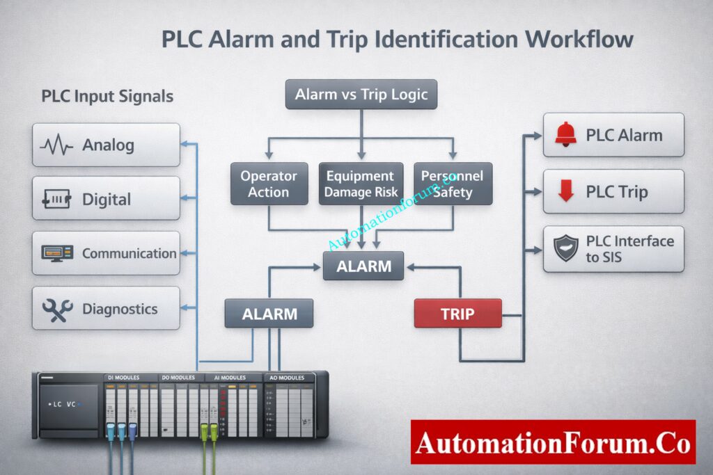
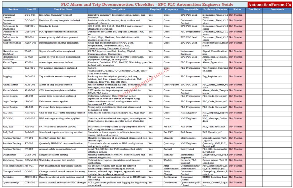
This document outlines a PLC-focused, auditable process for creating, documenting, testing, and transferring PLC alarms and trips in EPC projects. It sets explicit rules for who is responsible for what, how often testing should happen, and what must be delivered to get rid of hidden trips, cut down on annoying alarms, and make sure that PLC and HMI always work the same way. The technique is for PLC automation engineers, HMI engineers, instrument engineers, and commissioning teams, and it helps with FAT, SAT, and commissioning tasks.
The purpose of this document is to establish a standardized PLC alarm and trip documentation procedure that:
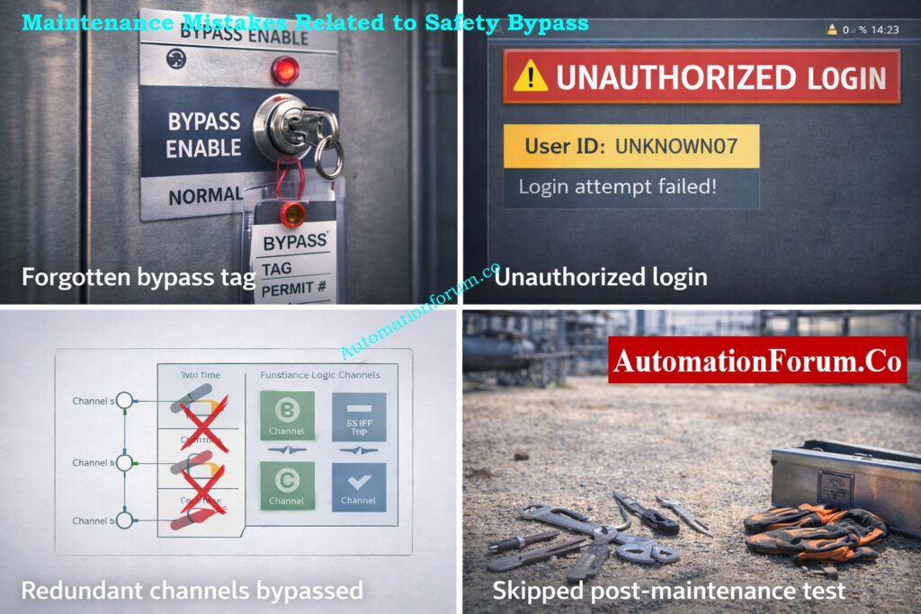
Eliminates undocumented logic and “hidden trips”
Prevents nuisance alarms and spurious trips
Ensures consistent PLC-HMI alarm behavior
Creates auditable FAT/SAT records
Enables smooth EPC handover to operations and maintenance
This procedure is written from a PLC automation engineer’s perspective, focusing on PLC code, tags, logic, testability, and traceability not plant operations theory.
Refer the below link for the Alarm & Trip Setpoint List in Instrumentation Engineering: The Most Critical Document for Plant Safety
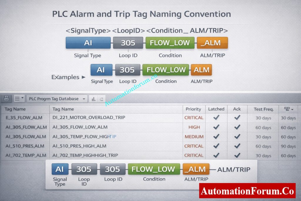
Each PLC alarm or trip tag shall include tag name, description, priority, acknowledgement requirement, latching behavior, test frequency, owner discipline, bypass permission, PLC address, data type, fail-safe state, and engineering comments. No alarm or trip shall be accepted without a completed attribute record.
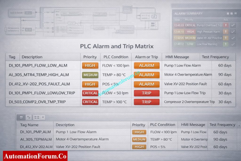
The alarm and trip matrix shall be maintained as the single source of truth for all PLC alarms and trips. Any PLC logic, HMI alarm, or test case without a corresponding entry in the alarm matrix is not permitted.
Alarm messages shall be short, clear, and action-oriented. Messages shall identify the equipment and condition without abbreviations that operators may misinterpret. Alarm logic shall not be implemented in the HMI. The HMI shall only display, acknowledge, and log PLC-generated alarms.
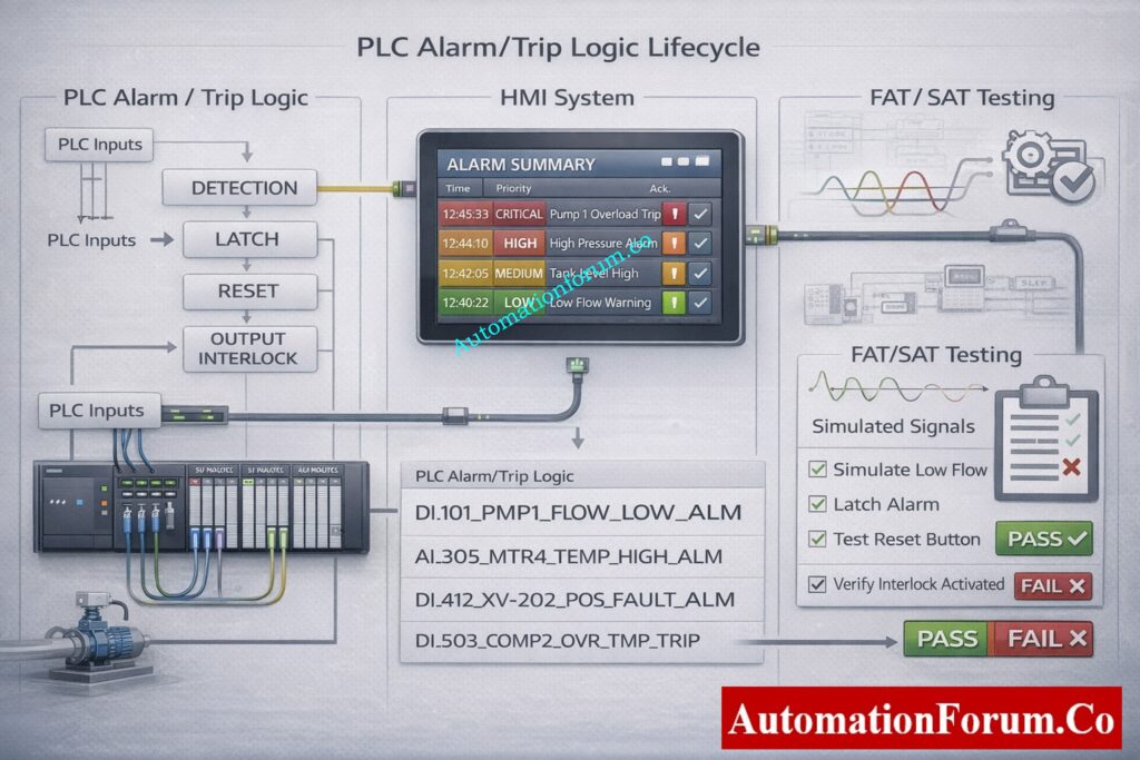
Functional Test Procedure (FAT / SAT) – Test Cases & Evidence
Before testing, look over the approved alarm matrix.
Check that the instruments are calibrated and that the signals are correct.
Use calibrated sources or PLC forcing to make alarm and trip circumstances happen.
Check the PLC’s detection time, latch behavior, and interlock logic.
Confirm final output actions such as motor stop or valve closure.
Verify HMI message text, priority, audible alarm, and acknowledgement behavior.
Verify alarm logging, timestamps, and operator identification.
Get things back to normal and check to see whether the reset works.
Write down the results and get the witness to sign off.
Standard FAT and SAT Test Case Structure
A documented test case that includes the test case ID, tag name, objective, preconditions, test procedures, expected results, actual results, tester name, date, and witness signature must be used to test each alert and trip. Testing without written evidence is not acceptable.
Change Control, Post-Maintenance Validation and Regression Testing
Any maintenance activity affecting PLC logic, field instruments, wiring, or I/O shall require re-testing of affected alarms and trips before returning the equipment to service. Results shall be recorded and approved by commissioning or maintenance engineering.
Mandatory Documentation & Archiving Rules
All test results must be recorded no verbal acceptance.
Store records in document control / EDMS with revision control.
Each record must include:
Date & time
PLC program version
Tester name & signature
Pass / fail status
Observations & corrective actions
Typical filenames:
PLC_Alarm_Matrix_vX.xlsx
PLC_Trip_Test_Record_YYYYMMDD.pdf
PLC_Post_Maintenance_Test_YYYYMMDD.pdf
Change Control Requirements
Any modification to alarm or trip logic shall follow formal change management. The change record shall include reason for change, affected tags, impact assessment, updated test results, revised alarm matrix, and approval from the EPC PLC lead. Version numbers shall be incremented for every approved change.
Download: PLC Alarm & Trip Test Checklist and Templates
This Excel checklist gives EPC projects a disciplined and verifiable way to record, test, and hand over PLC alarms and trips. It makes sure that the PLC and HMI always work the same way, gets rid of undocumented logic, and helps with FAT, SAT, and commissioning tasks. It was made for PLC automation engineers and helps make sure that everything works right and that the EPC handover is clean.
Download the PLC Alarm & Trip Test Checklist (automationforum.co) and join our professional forum at automationforum.co to access EPC-grade PLC templates, alarm matrices, and peer-reviewed practices.
PLC alarm and trip logic changes shall be restricted to authorized personnel only. Forcing of alarm or trip tags shall be logged with user name, date, time, and reason. Remote access to PLC systems shall comply with company cybersecurity policies.
PLC alarms and trips shall not be treated as replacements for SIS protections. All safety-related PLC logic must be clearly identified and coordinated with SIS design. For long-term operation to be reliable, documenting, tagging, and testing must be done on a regular basis.
PLC alarms and trips should never be used instead of SIS protections. All PLC logic that has to deal with safety must be explicitly marked, written down, tested, and included into the SIS design. For safe and reliable plant operation, paperwork and testing must be done on a regular basis.
A PLC alarm is a programmed condition that finds an abnormal state of equipment or process. It tells the operator to take action through HMI or DCS. Alarms can be latched or not latched, and you normally have to recognize them.
What is the alarm and trip schedule?
An alarm and trip schedule is a documented list of all PLC alarms and trips with conditions priorities actions and test frequency. It is commonly maintained as an alarm or trip matrix. It is used during design testing commissioning and maintenance.
How does a PLC work step by step?
A PLC reads inputs from field devices executes the control logic and updates outputs. It communicates status to HMI or DCS and repeats this scan continuously. The entire scan cycle runs in milliseconds.
What are the safety precautions for PLC?
Use proper grounding shielding and surge protection for PLC systems. Apply access control backups and change management for programs. Always follow lockout tagout procedures during testing and maintenance.
What are 5 safety precautions?
Ensure proper earthing and power protection. Apply lockout tagout before panel work. Restrict PLC program access with passwords. Verify wiring and I O before energizing. Maintain updated backups and documentation.
What are the 4 steps of PLC?
The PLC performs an input scan to read signals. It executes the control program logic. It updates output signals to field devices. Communication and diagnostics complete the scan cycle.
Why Resolution in PLCs Matters in Industrial Automation
If you design, commission, or maintain control systems, understanding resolution in PLCs is non-negotiable. Resolution is the smallest change a PLC can detect or represent. It determines how precisely you can measure temperature, pressure, speed, position, or any analog signal. For instrumentation and calibration engineers (like many readers here), resolution affects scaling, alarm accuracy, PID tuning, and traceability of calibration certificates.
This guide is written for automation engineers, instrumentation technicians, and controls specialists. It’s SEO-optimized for queries like PLC resolution, 16-bit unsigned vs signed, analog input resolution, and how to calculate PLC step size. You’ll get clear formulas, worked examples (digit-by-digit), practical tips, and common mistakes to avoid.
What Is Resolution in PLCs? (Core Concept Explained)
Definition of Resolution in PLC Systems
Resolution = smallest increment the PLC can represent.
It depends entirely on the number of discrete steps a value can take – which in turn depends on the number of bits used to store that value.
Resolution (step size) = (Max Value − Min Value) ÷ Number of steps
And:
Number of steps = 2ⁿ where n = number of bits.
Resolution vs Accuracy vs Precision in PLC Systems
Resolution, accuracy, and precision are often confused in PLC and instrumentation systems, but they are not the same.
Resolution defines the smallest detectable change in a signal based on bit depth. Accuracy indicates how close the measured value is to the true value. Precision refers to repeatability of measurements.
A PLC can have high resolution but poor accuracy if the sensor or calibration is incorrect. Likewise, high accuracy with low resolution results in coarse signal steps. For reliable control, all three must be considered together.
A common sample: a 12-bit sensor that measures 0 °C to 100 °C.
Number of steps = 2¹² = 4096.
Resolution = (100 − 0) ÷ 4096.
Let’s compute that carefully:
4096 × 0.0244140625 = 100.0000000 (so resolution is exact to many decimals)
Therefore resolution = 0.0244140625 °C per bit (rounded commonly to 0.02441 °C/bit)
This means the PLC/ADC cannot distinguish temperature changes smaller than ~0.02441 °C.
16-Bit Unsigned Resolution Example (0–10 V Analog Input)
A common PLC input is 0–10 V mapped to a 16-bit unsigned integer.
Number of steps = 2¹⁶ = 65,536.
Resolution = (10 V − 0 V) ÷ 65,536.
Compute:
10 ÷ 65,536 = 0.000152587890625 V per bit (Rounded: 0.00015259 V/bit)
So each increment in the ADC raw value represents ~152.6 μV.
16-Bit Signed Resolution for Bipolar Signals
If a signed 16-bit integer is used for a bipolar signal (for example −5 V to +5 V mapped to signed counts), the effective symmetric step count per side is 2¹⁵ = 32,768.
If you map −5 V to +5 V on a signed 16-bit:
Steps per side = 32,768
Resolution = (5 V − (−5 V)) ÷ 65,536 = 10 ÷ 65,536 = same as unsigned example above.
However, when you reason per side, you often think in ±5 V mapped to −32,768 … +32,767 counts, which halves the positive/negative bucket for sign encoding reasons.
Refer the below link for the PLC Raw Count Calculator: Comparison with PLC Internal Scaling Blocks, Real-World Use Cases and Practical Benefits
Practical point: If your signal is inherently always positive (0–100), using signed integers wastes half the useful counts. For best resolution use unsigned for strictly positive ranges and signed for bipolar signals.
Analog Resolution in PLCs and ADC Considerations
How PLC ADC Converts Analog Signals to Digital Values
Impact of PLC Resolution on PID Control Performance
When you connect a physical sensor (RTD, thermocouple with transmitter, 4–20 mA loop, or 0–10 V) the ADC inside the PLC converts that voltage/current into discrete digital counts.
Effective Number of Bits (ENOB) in PLC Analog Inputs
Even a 16-bit ADC can be effectively fewer bits of usable resolution if noise or poor wiring degrade the SNR. In practice, 16-bit resolution often delivers 12–14 bits of effective bits (ENOB) in noisy industrial environments unless you manage wiring and filtering carefully.
PLC resolution and sensor resolution are independent parameters. The overall system resolution is always limited by the weakest element.
If a sensor provides only 0.5 °C resolution, using a 16-bit PLC analog input will not improve measurement accuracy. Conversely, a high-resolution sensor connected to a low-resolution PLC input wastes sensor capability.
Effective system resolution = minimum(sensor resolution, ADC resolution, signal noise limit).
Resolution tells you how little a change in a signal can be seen, and scan time tells you how often the PLC reads that change.
A PLC with high resolution and slow scan time might not pick up signals that change quickly. Also, if the scan duration is fast but the resolution is low, the measurements will be wrong.
When dealing with dynamic processes, you need to choose both the resolution and the sample rate at the same time to make sure the control is stable.
Analog output resolution determines the smallest change a PLC can apply to actuators such as control valves or variable speed drives.
For a 16-bit analog output with a 0–10 V range, each step represents approximately 0.00015 V. Low AO resolution causes stepwise output changes, leading to valve hunting or unstable speed control.
High-resolution analog outputs are critical for precise flow, pressure, and speed control applications.
Common PLC Resolution Mistakes and How to Avoid Them
Using signed vs unsigned incorrectly. If your signal is always positive, using signed storage loses half the dynamic range.
Not accounting for ADC offset or calibration error. Always calibrate end-points and include offset/gain compensation.
Rounding too early. Round only for display. Keep full precision internally until final output.
Expecting theoretical resolution equals usable resolution. Noise, grounding, and ADC ENOB reduce usable bits. Improve wiring and filtering to raise effective bits.
Scaling mistakes causing alarm thrashing. If alarm deadbands are smaller than step size, alarms may oscillate. Set alarms with hysteresis at least ± one or two counts.
Treating counts as engineering units in documentation. Always show both raw counts and engineering units in calibration and handover docs.
Impact of PLC Resolution on PID Control Performance
PLC resolution has a direct impact on PID loop stability and performance. Low resolution causes quantization errors, resulting in step changes instead of smooth control output.
Poor resolution can lead to limit cycling, oscillations, and excessive valve movement. High-resolution inputs and outputs allow finer PID adjustments, smoother control action, and reduced mechanical wear.
For tight control loops, resolution should be significantly smaller than the smallest process change requiring correction.
Practical Limits to PLC Resolution in Real Industrial Plants
In real industrial environments, usable PLC resolution is often lower than theoretical resolution.
Electrical noise, poor grounding, long cable runs, EMI, temperature drift, and improper shielding reduce effective number of bits (ENOB). As a result, a 16-bit input may behave like a 12-bit system in harsh conditions.
Good wiring practices, proper grounding, shielding, and signal filtering are essential to achieve usable resolution.
Steps per side = 2¹⁵ = 32,768. If mapping −10 V…+10 V to signed counts, resolution = 20 ÷ 65,536 = same as unsigned full span — but positive/negative split matters for indexing and alarms.
PLC resolution varies by manufacturer and analog module design.
Many Siemens PLC analog inputs scale 0–10 V to 0–27,648 counts, while Allen-Bradley modules often use the full 16-bit range. Schneider and Yokogawa modules may use different internal scaling and filtering methods.
Always refer to vendor manuals to confirm raw value ranges before scaling and calibration.
Include raw counts + mapped engineering units in punch list.
State ADC bit depth and signed/unsigned setting.
Provide calibration certificate with end-point counts and dates.
Specify alarm deadband relative to step size.
Note ENOB or measured noise floor if available.
Resolution is the bridge between the physical world and your PLC’s digital brain.
Choose the right bit depth, use the correct signed/unsigned representation, document scaling precisely, and always validate usable resolution in the field (not just on paper). If you do those four things, your control loops will be more accurate, alarms more stable, and calibration records more defensible.
Resolution plays a critical role in alarm and trip system design. Alarm setpoints must account for resolution step size to avoid nuisance alarms or missed trips.
If alarm thresholds are closer than one resolution step, the PLC may not detect the condition reliably. Proper alarm deadbands and safety margins must always consider PLC resolution.
This is especially important for safety instrumented systems and shutdown logic.
PLC resolution and HMI display resolution are not the same.
An HMI may display values with many decimal places, but the actual PLC resolution limits the true measurement. Displaying extra decimals does not increase accuracy or resolution.
Engineering decisions should always be based on PLC resolution, not visual display precision.
Key Rule: PLC resolution determines what the controller can detect, accuracy determines correctness, and display decimals only affect appearance not control quality.
Frequently Asked Questions (FAQ) on Resolution in PLCs
What is resolution in a PLC?
Resolution in a PLC is the smallest change in an input or output signal that the PLC can detect or represent. It depends on the number of bits used to store the value and the signal range.
How do you calculate PLC resolution?
PLC resolution is calculated using the formula: Resolution = (Maximum Value − Minimum Value) ÷ 2ⁿ, where n is the number of bits used by the PLC or ADC.
What is the resolution of a 16-bit PLC?
A 16-bit PLC has 65,536 discrete steps (2¹⁶). The actual resolution depends on the signal range—for example, a 0–10 V signal has a resolution of approximately 0.00015 V per bit.
What is the difference between signed and unsigned resolution in PLCs?
Unsigned integers use the full range for positive values (0 to 65,535), giving better resolution for unipolar signals. Signed integers split the range into positive and negative values, reducing usable resolution per side.
Why is PLC resolution important in analog signals?
PLC resolution determines how accurately analog signals like temperature, pressure, or flow can be measured. Higher resolution allows detection of smaller signal changes, improving control accuracy and stability.
What happens if PLC resolution is too low?
Low resolution causes large step sizes, leading to poor measurement precision, unstable PID control, inaccurate alarms, and scaling errors in analog signals.
Which PLC data type gives better resolution?
For positive-only signals, unsigned integers give better resolution because they use the full numeric range. Signed integers are better for signals that can go positive and negative.
What is the resolution of PLC analog?
The smallest change in an analog signal that the PLC can see is called PLC analog resolution. It depends on the ADC’s bit depth and signal range, which is (Max − Min) ÷ 2ⁿ.
What is 16-bit resolution?
The signal is split into 65,536 separate steps (2¹⁶) when it has a 16-bit resolution. This makes it possible to find very minor changes in analog signals, which makes measurements more accurate.
What is resolution in a control system?
In a control system, resolution is the smallest change in a variable that the system can measure or control. Higher resolution makes it easier to control things and gives you more accurate feedback.
What does 12-bit resolution mean?
The 12-bit resolution breaks the signal range down into 4,096 steps (2¹²). Each step is a set amount that tells you how precise the signal may be measured or regulated.
What is a 24-bit resolution?
With 24-bit resolution, you can measure very minor changes in signals with 16,777,216 steps (2²⁴). It is often employed in systems for collecting data and high-precision instruments.
Which is better, 10-bit or 12-bit?
12-bit resolution is superior since it has four times as many steps as 10-bit resolution. This makes the step size lower, the accuracy higher, and the control accuracy better.
What is the difference between 12-bit and 14-bit resolution?
With 12 bits of resolution, there are 4,096 steps. With 14 bits of resolution, there are 16,384 steps. The 14-bit system offers four times finer resolution and more precise signal measurement.
What is resolution in process control?
Resolution in process control refers to the smallest change in a process variable that the control system can detect or adjust. Higher resolution improves stability, accuracy, and control performance.
Refer the below link to Optimize PLC Scan Time Fast
Why Valve Actuator Sizing Is Critical in EPC Instrumentation Projects
Sizing the valve actuator is one of the most risky design tasks in EPC instrumentation and control projects. If the actuator is the wrong size, the valve may stop working, the actuator motor may overload, the gearbox parts may wear out too quickly, or the shutdown valves may completely fail during an emergency.
This guide provides a deep technical explanation of valve actuator sizing, aligned with how the Valve Actuator Torque, Safety Factor & Gear Ratio Calculator works in practice. The article is for EPC instrumentation engineers, control engineers, and commissioning technicians who work with ball valves, butterfly valves, globe valves, and linear control valves.
Why Valve Actuator Sizing Requires More Than Datasheet Torque
In principle, valve makers give a torque number that looks like it would be enough for choosing an actuator. The actuator sizing calculator takes this into account by looking at more than just valve torque when figuring out how much torque to use.
In EPC projects, valves are exposed to:
Dirt, dust, and corrosion
Packing tightening over time
Temperature variation and thermal expansion
Infrequent operation (especially for shutdown valves)
Because of this, real operating torque is always higher than nominal datasheet torque. Industry standards such as ISO 9359 and NORSOK explicitly recognize this and recommend adding allowances and safety margins.
The actuator sizing calculator takes this into account by looking at more than just valve torque when calculating the size of the actuator.
NORSOK guidelines often recommend 10–20% additional torque for harsh service. This is entered as a separate torque component in the calculator, not hidden inside the safety factor.
Safety Factor
The safety factor ensures long-term reliability by accounting for:
Typical EPC Applications of This Valve Actuator Sizing Methodology
This actuator sizing methodology can be applied across multiple phases of an EPC project and throughout the valve life cycle.
FEED and Detailed Engineering Phase
During front-end and detailed engineering, this approach helps establish realistic actuator torque requirements based on valve data, service conditions, and design margins. It supports early standardization and prevents late design changes during procurement.
Actuator Datasheet Preparation
You can immediately copy the calculated needed torque, safety factor, and gearbox ratio into actuator datasheets. This makes ensuring that vendor quotes are based on consistent and technically sound sizing standards.
Vendor Bid Evaluation and Technical Clarification
The size findings give you a straightforward way to compare vendor bids. You can objectively check actuator torque ratings, gearbox efficiency, and proposed gear ratios against the projected needs. This lowers the chance of making a wrong choice.
FAT and SAT Verification
You can use the size calculations to check the performance, torque capabilities, and stroke time of the actuator during factory and site acceptance testing. Any difference between what the design was meant to do and what it really does can be found early.
Brownfield Valve Automation Projects
This sizing method lets engineers look at existing valves again using current process conditions and choose the right actuators without having to rely on old or incomplete paperwork for refit or automation projects.
This structured approach helps maintain consistency between design calculations, procurement specifications, and commissioning performance, reducing operational risks and rework.
Before approving the actuator selection, the following checks should be completed to avoid commissioning and long-term reliability issues.
Verification of Torque Components
Verify that valve operating torque, packing or friction torque, and environmental allowances are all included in the calculation. Using only the valve datasheet torque can result in undersized actuators.
Validation of Safety Factor Application
Confirm that the safety factor is applied to the total combined torque and not only to the valve torque. The chosen value should fit the valve’s job, like controlling service or shutting down in an emergency.
Confirmation of Gearbox Efficiency Inclusion
Make sure that the computation includes gearbox efficiency as a loss. To prevent underestimating actuator torque needs, lower efficiency, especially for worm gearboxes, must be taken into account.
Review of Torque Margin
Make sure that there is enough extra torque above what is needed. For control valves, a minimum of 20% is usually required, and for safety-critical valves, a higher percentage is usually advised.
Verification of Output Speed and Stroke Time
After choosing a gearbox, check the actuator output speed again to make sure that the times for opening and closing the valve match safety and process standards without generating shock or instability.
Frequently Asked Questions on Valve Actuator Sizing
What is the formula for valve sizing?
The flow equation, which relates flow rate, pressure drop, fluid density, and valve coefficient (Cv or Kv), is often used to figure out the size of a valve. The basic equation is Q = Cv × √(ΔP / SG). The exact formula changes depending on whether the fluid is a gas, liquid, or steam.
The size of a PSV is depending on its relieving capacity, set pressure, permitted overpressure, and the parameters of the fluid. To find the right orifice area, you use standard equations from API 520. The chosen PSV must be able to handle the desired flow without going above the maximum pressure limitations.
An actuator sizing program is a tool that helps you figure out how much torque or thrust an actuator needs. It takes into account the valve’s torque, friction, safety factor, and how well the gearbox works. The program tells you what size actuator and gear ratio you need.
To choose the proper actuator, you need to figure out how much torque or thrust is needed at the valve stem and compare it to the actuator’s continuous rated output. You also need to think about the type of valve, the circumstances of service, the duty cycle, and the speed requirements.
To find the size of an actuator, add up the valve torque, friction, and environmental allowances, and then add a safety factor. To figure out the minimal continuous actuator torque needed, we take into account the losses in gearbox efficiency.
What is a 3 point actuator?
A 3 point actuator is an electrically operated actuator that has three signals: open, close, and common. Instead of using an analog position signal, it adjusts the valve in small steps based on control inputs.
Refer the below link to Try PID tuning Simulation Tool for Engineers
Why Safety Bypass And Override Matter For Instrumentation Maintenance
Safety bypass and override activities are among the most critical and high-risk tasks performed by maintenance and reliability engineers in process plants. In oil and gas, chemical, power, and other hazardous industries, Safety Instrumented Systems are designed as independent protection layers that prevent catastrophic events such as explosions, toxic releases, fires, and major equipment damage.
Industrial Incidents Caused By Uncontrolled Safety Bypasses
History has repeatedly shown that many serious industrial incidents did not occur because safety systems were poorly designed, but because they were bypassed, overridden, or left disabled during maintenance. Forgotten bypasses, undocumented overrides, and uncontrolled temporary workarounds have resulted in loss of containment, environmental damage, and fatalities.
For maintenance engineers, bypassing a safety function is sometimes unavoidable. Proof testing, transmitter replacement, valve maintenance, and troubleshooting often require temporary suspension of a safety function. IEC 61511 safety bypass and override requirements exist to ensure these necessary activities are performed in a disciplined, controlled, and traceable manner without compromising plant safety.
This article explains how maintenance teams should manage safety bypass and override activities in real plant conditions, focusing on what must be done in the field, not academic interpretations of the standard.
Understanding Safety Bypass And Override In A Safety Instrumented System (SIS)
Definition Of Safety Instrumented System Bypass And Safety Override
In a Safety Instrumented System, a safety bypass refers to the intentional temporary disabling of a safety instrumented function while the plant continues operating. The input signal may still be visible, but the logic solver is prevented from executing the shutdown or protective action.
A safety override typically forces a device or logic state to a predefined value regardless of actual process conditions. In practice, both bypass and override remove the automatic protective action of the SIS and therefore carry similar risks.
Difference Between Temporary Bypass And Permanent Override
The most important distinction is between temporary bypass and permanent override.
A temporary bypass is applied for a clearly defined maintenance purpose and is expected to be removed immediately after the task is completed. Some examples are skipping a pressure transmitter during calibration or turning off a shutdown valve during stroking tests.
A permanent override takes away the safety feature from normal functioning. This is not a maintenance task; it is a design change that needs a comprehensive safety analysis and management of change.
The fundamental safety philosophy behind IEC 61511 is that each protection layer must remain effective throughout the plant lifecycle. When a safety function is bypassed, the risk reduction it provides is temporarily lost.
Uncontrolled bypass defeats the purpose of having a Safety Instrumented System. If it were easy or casual to bypass safety layers, operators would not know they were running the plant without them, which would give them a false sense of security.
IEC 61511 safety bypass and override controls are intended to ensure that:
Bypass is deliberate, not accidental
Bypass is visible to operations
Bypass is authorized by responsible personnel
Bypass is time-limited
Bypass is compensated by other risk reduction measures
The standard emphasizes that procedures alone are not sufficient. Technical controls, access restrictions, alarms, and traceability must support administrative controls.
Roles Of Maintenance, Operations, SIS Engineers and Management
Before any safety bypass is applied, maintenance engineers must evaluate the process risk associated with disabling the safety function.
The risk assessment should consider:
What hazard is normally controlled by this safety function
What could happen if the hazard occurs during the bypass period
How likely the initiating event is under current operating conditions
What consequences could result if protection is unavailable
Safety Bypass Permit Content And Approval Workflow
The assessment should also identify existing independent protection layers such as relief valves, alarms, operator intervention, or physical barriers.
If the residual risk cannot be reduced to an acceptable level using compensatory measures, the bypass must not be applied and alternative maintenance methods should be considered.
This evaluation does not need to be a full hazard study, but it must be documented, reviewed, and approved before proceeding.
Integration With Permit-to-Work And Management of Change
Safety bypass must never be a single-person decision. Authorization usually requires more than one role:
Maintenance engineer Suggests the bypass, defines its scope, lists the specific signals or final elements that will be affected, and outlines the intended compensatory procedures.
Operations Checks to see if the procedure is ready, makes sure that the current operating conditions make the temporary drop in protection acceptable, and agrees to any operational limits.
SIS or safety engineer Checks that the proposed bypass won’t accidentally turn off other levels of security, makes sure that the bypass method is technically sound, and finds any tests or diagnostics that need to be done.
Plant Management or Delegated Authority
Gives the last word on bypasses that are very risky or go beyond normal maintenance windows.
A formal permission or SIS bypass authorization form should be used to record bypass approval. The permit must say clearly:
Which safety function is bypassed
Why the bypass is required
Start and end time
Compensatory measures
Authorized personnel
Only people who have been trained and given permission should be able to turn on or off the bypass.
Bypass Implementation and Control System Practices (SIS Maintenance Practices)
Control systems should be set up and designed in a way that makes safe bypass management possible.
Some important things to do are:
HMI Indication And Visibility Of Bypassed Safety Functions
The operator interface should explicitly show any active bypass or override, name the function that is affected, and name the person who put it in place.
Alarm Management For Active Bypasses
When you use a bypass, it should set off a different alarm and put it at a high enough priority level so it can’t be easily silenced. The alarm should keep going off until the bypass is taken away and the function is checked.
Access Control Using Passwords, Roles And Key Switches
Only authorized roles should be able to apply or remove bypasses. For high-risk tasks, use accounts with passwords, role-based permissions, or physical key switches.
Logging, Traceability And Audit Records
It is important to automatically log bypass activities with the user ID, timestamp, cause, and predicted expiration. These logs help in audits and investigations of incidents.
Selective Bypass To Preserve Redundancy
If the architecture enables it, only bypass the least amount of elements needed. For example, bypass a single channel rather than the entire trip logic. Selective bypass reduces the reduction in safety integrity and preserves available redundancy.
Fail-Safe Design Of Bypass Mechanisms
Ensure that the control system design returns automatically to a safer state on loss of communication or if the bypass control fails. The bypass mechanism itself must be subject to the same engineering rigor as other SIS changes.
Bypass status must be visible to operators at all times, not hidden in maintenance menus.
Every safety bypass needs to have a set time limit.
The longer a bypass is open, the more dangerous it becomes. If a bypass lasts longer than the maximum time allowed, it should need to be re-authorized.
Shift Handover Review And Re-Authorization Rules
During shift handovers, maintenance crews should keep an eye on the status of bypasses and review any active bypasses.
If repair can’t be done in the period that was agreed upon, the bypass needs to be looked at again, not automatically extended.
Returning The Safety Function To Service (Instrumentation Maintenance Safety)
It should be a regulated, documented process to remove a bypass that checks the function before normal operation can start again.
Step 1: Verifying Physical Restoration Of Instruments And Valves
Check that the wiring, instruments, and final items are all properly reconnected and reinstalled.
Step 2: Restoring Normal Signals And Removing Test Connections
Re-enable inputs and take off any test wiring or connections required for maintenance.
Step 3: Functional Testing And Validation Of Safety Logic
Do a functional test to show that the safety logic and final items work as they should. Tests should be authentic and, if it’s safe to do so, they should be like a real demand.
Step 4: Monitoring Operation After Bypass Removal
After taking it out, check to see if it works as expected under typical process circumstances. Use diagnostics to look for hidden problems.
Step 5: Documentation And Communication With Operations
Put the test results, the time, and the name of the person who took down the bypass in the permit record. Tell operations and plant management that the safety function is back in place.
These processes are necessary to meet the safety bypass and override requirements of IEC 61511 and to make sure that risk has not been left unmanaged by mistake.
You can’t finish the job unless the safety function is fully working and tested.
Integrate bypass control into permit-to-work systems.
Use control system features to enforce authorization and time limits.
Design SIS to minimize the need for bypass where possible.
Schedule maintenance during low-risk operating periods.
Review bypass history to identify recurring issues.
Treat every bypass as a temporary degradation of plant safety.
Ultimate Maintenance Checklist – Prevent Failures Before They Happen- Maintenance Checklist
Disciplined Safety Bypass Management Under IEC 61511
IEC 61511 safety bypass and override requirements exist to protect plants from the hidden dangers of disabled safety systems. For maintenance and reliability engineers, disciplined bypass management is not just a compliance activity, it is a core professional responsibility.
When safety bypasses are properly justified, authorized, compensated, monitored, and removed, plants can maintain high availability without sacrificing protection. Poor bypass practices, on the other hand, expose facilities to unacceptable risk and erode trust in maintenance operations.
Strong safety bypass management demonstrates technical competence, operational discipline, and commitment to protecting people, assets, and the environment.
IEC 61511 is an international standard that defines how Safety Instrumented Systems are specified, designed, operated, and maintained to reduce process safety risks. It focuses on preventing hazardous events in industries such as oil and gas, chemicals, and power. The standard ensures risks are reduced to a tolerable level throughout the plant lifecycle.
What is the meaning of bypassing safety controls?
Bypassing safety controls means temporarily disabling or overriding a safety function to allow maintenance, testing, or troubleshooting. During a bypass, the safety system cannot automatically protect the process from hazardous conditions. Because risk increases, bypassing must be authorized, time-limited, and supported by compensatory measures.
When must functional safety assessment be done according to IEC 61511?
Functional safety assessment must be performed at key stages of the Safety Instrumented System lifecycle. This includes after design, before commissioning, after modifications, and periodically during operation. The assessment verifies that the safety system meets its intended safety performance.
What is the difference between SIF and SIS?
A Safety Instrumented Function is a single protective function designed to reduce risk, such as a high-pressure shutdown. A Safety Instrumented System is the complete system that implements one or more SIFs, including sensors, logic solvers, and final control elements.
What are the 5 levels of safety?
The five common levels of safety include inherent process safety, basic process control systems, alarms and operator intervention, Safety Instrumented Systems, and physical protection or emergency response. Each layer works independently to reduce risk. If one layer fails, the next provides protection.
A Safety Instrumented Function is an automatic safety action designed to bring the process to a safe state when dangerous conditions occur. It uses sensors, logic, and final elements to prevent accidents. Each SIF is assigned a Safety Integrity Level based on risk reduction requirements.
Refer the below link for the Advanced Field Instrument Reliability & Cyber-Secure Maintenance Checklist


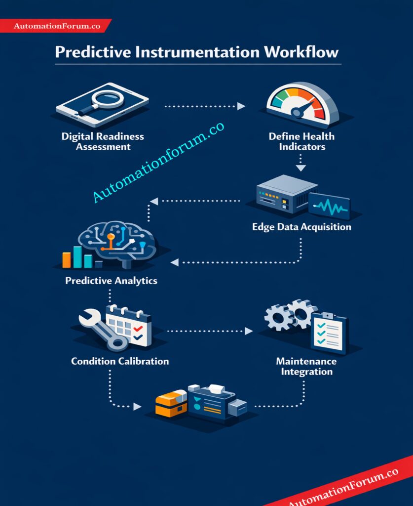

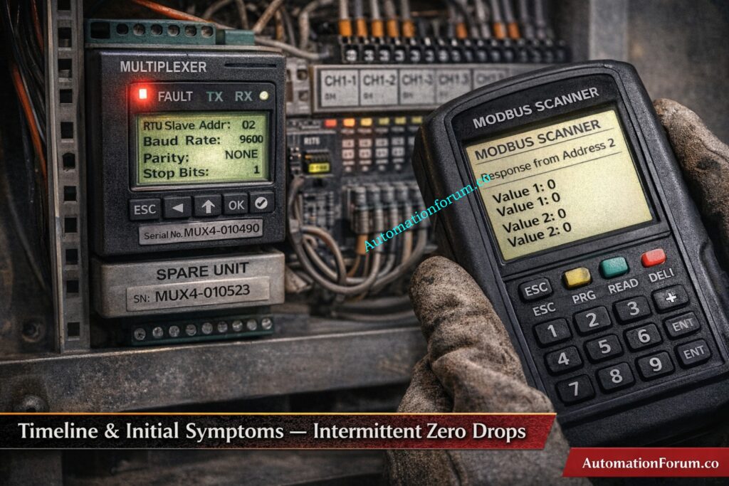

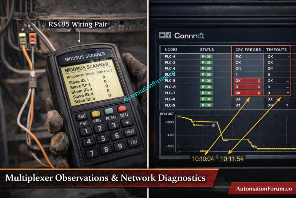
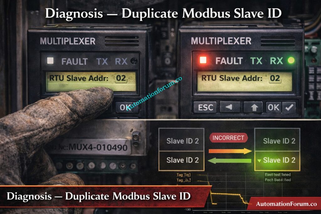
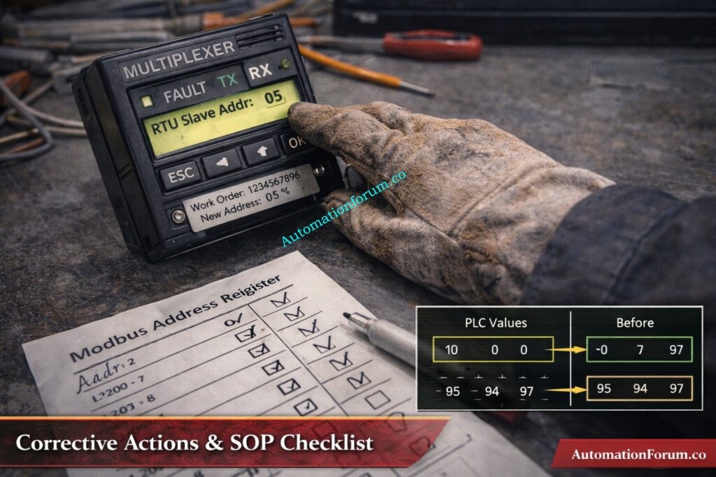


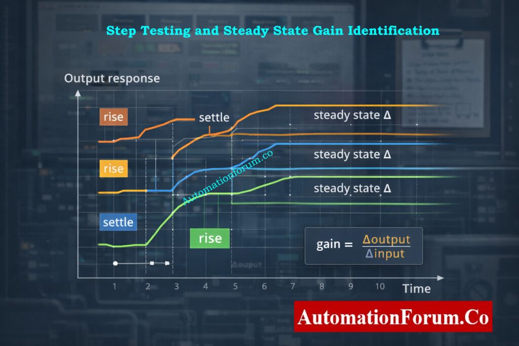
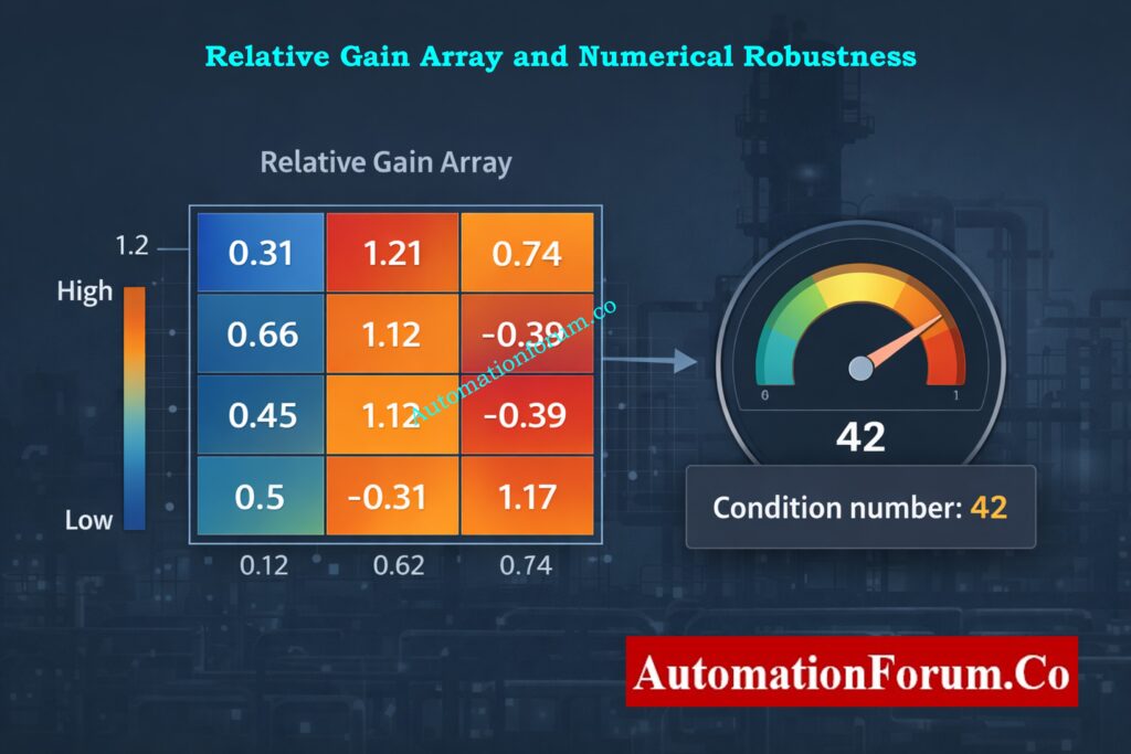
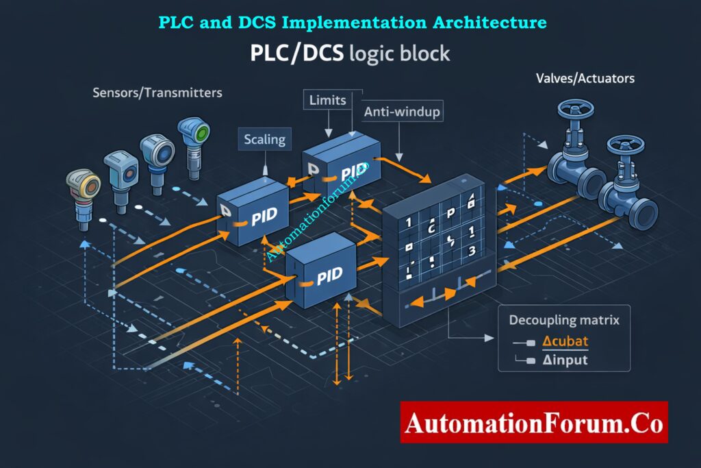
 1")