Why Automation Engineers in Process Industries Should Master PLC Programming Basics
This short, advanced quiz is for automation engineers who work in process industries and want to learn the foundations of PLC programming. The questions are based on real-life situations you may see on the plant floor and cover ladder logic, function blocks, scan cycle behavior, HMI integration, and fieldbus communications. Take it to test your talents, find out what you don’t know, and get results you may share with your coworkers to push them.
Test Your PLC Programming Basics Skills – Advanced Quiz for Process Industries
Sharp, useful, and ready for the test This quiz will help you improve your ability to debug, structure code, and think about control strategies in high-stakes process situations. Do it all at once, compare scores, and receive a summary that you may print out to identify areas that need quick improvement. Now.
Choosing the wrong PLC data type is one of the quiet but deadly mistakes in automation projects. A flow transmitter stored as an INT loses decimal resolution. A totalizer stuck in a 16-bit integer overflows in a month. Lots of STRING tags mean sluggish memory use and longer backups. These aren’t academic problems they cause incorrect displays, false alarms, unexpected trips, and frustrating downtime.
PLC data types aren’t just a syntax detail; they determine numeric accuracy, memory footprint, scan time performance, and how easy the system is to maintain. Good PLC data type selection prevents overflow, preserves precision for control loops, and makes diagnostics fast and predictable. In this article you’ll get a clear, practical walkthrough of the key PLC programming data types (PLC BOOL INT DINT REAL and more), real-world usage patterns, common PLC programming mistakes, and hardened best practices for PLC data type selection and PLC memory optimization. Read on for actionable guidance that helps you design reliable, high-performance automation logic.
Why PLC Data Types Matter in Real-World Automation
Correct data type choice affects multiple dimensions of a control system:
Accuracy of measurements: wrong numeric type truncates or rounds process values (temperature, flow, pressure).
PLC scan time: heavy types (floating point, long strings) and conversions increase CPU load and latency.
Memory usage: data types determine tag size; inefficient choices bloat memory and slow backups.
System reliability: overflow, conversion errors, or lost precision create logic faults and mis-actions.
Troubleshooting speed: consistent, sensible types make it easy to figure out what’s wrong and why.
When engineering teams don’t think about data types until the last minute, they typically have to do a lot of expensive rework during commissioning or lose production later on.
Common PLC Programming Problems Caused by Wrong Data Types
Real examples you’ll run into:
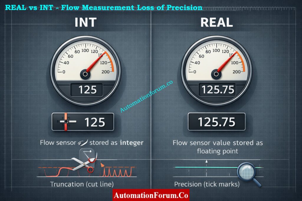
INT vs REAL for flow values: When you store a flow of 125.75 L/min in INT, it gets cut off at 125, which gives PID the wrong input and causes a steady-state error.
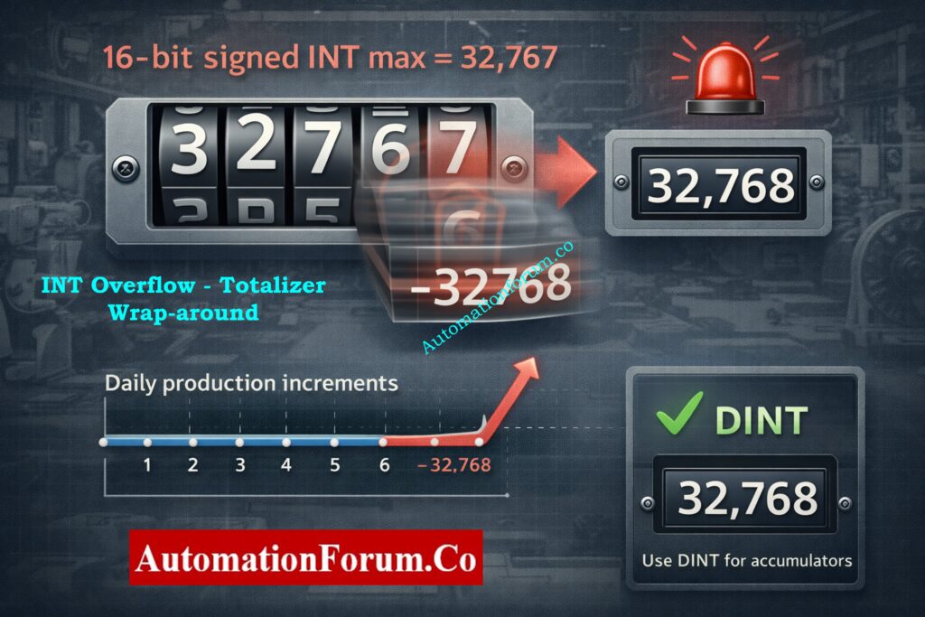
INT overflow in totalizers: When totalizers have an INT overflow, the maximum value for a 16-bit signed INT is 32,767. A production counter that goes over that flips negative or wraps, which messes up logs.
Excessive STRING usage: using STRING for anything other than user messages increases memory use and slows tag scans and backups.
Misuse of WORD vs DWORD: mapping device registers into WORD when device returns 32-bit values loses half the data or misaligns bitfields.
Consequences are practical: wrong control actions, erratic HMI values, spiking PLC CPU, and confusing alarm patterns.
PLC Data Types Explained for Instrumentation and Control Engineers
This comprehensive guide explains the most commonly used PLC data types in industrial automation and instrumentation systems. It is written for instrumentation engineers, control engineers, PLC programmers, maintenance engineers, and automation professionals working with PLCs,DCS,SCADA, and Modbus based systems. Each type of data has a definition, size, value range, uses, examples from the real world, remarks, and tips for fixing problems.
Pump_Run equals TRUE when the motor starter feedback contact is energized.
Real World Notes
PLCs usually pack BOOLs into bytes or words for memory efficiency so a block of 8 BOOLs may share the same underlying byte. That means a single-byte write (from HMI or network) can inadvertently flip other bits if not handled atomically.
Many vendor toolchains support bit-level addressing (e.g., I:0/1), but communication protocols like Modbus often expose whole registers mapping and masking are needed.
For safety/interlocks, treat BOOLs as status flags only; avoid using them for arithmetic or accumulation.
Quick Diagnostic and Best Practice
Check for non-atomic writes and read-modify-write races when a single bit changes without warning.
Put logically relevant flags into a byte or word to make communication faster, but be careful when masking and unmasking bits in your code.
A byte is a data container that holds 8 bits of information.
Size
8 bits.
Value Range
0 to 255.
What It Stores
Small grouped flags, compact status information, simple encoded values.
Typical Applications
Device status bytes, communication data, simple codes returned by instruments.
Practical Example
A field device returns a status code between 0 and 200 stored in a single byte.
Real World Notes
Bytes are commonly used for compact status encoding and simple ASCII characters. They’re useful when reading/writing modbus registers that return 8-bit status bytes.
Watch BCD and ASCII encodings a value of 0x31 can mean ASCII ‘1’ (49 decimal) or the numeric 31 in BCD depending on vendor. Clarify encoding in device docs.
Byte arithmetic overflows wrap around explicit checks or use larger types when summing many bytes.
Quick Diagnostic and Best Practice
Always check to see if a byte is raw data, ASCII, BCD, or bit flags.
To get nibble-level information without making mistakes, use masking (byte & 0x0F).
A Word is a 16 bit unsigned integer. Naming conventions may vary between PLC vendors.
Size
16 bits.
Value Range
0 to 65535 unsigned.
What It Stores
Raw analog values, bit mapped registers, register based counters.
Typical Applications
Raw ADC counts from analog input modules, Modbus holding registers.
Practical Example
AI_raw equals 27648 read as a 16 bit word from an analog input module.
Real World Notes
Many field devices export 16-bit registers; interpreting them correctly is fundamental. If the sensor produces negative values it may be in two’s complement (signed) even if the documentation calls it a register.
Common use: store raw ADC counts (0–32767 or 0–65535) and then apply scaling (engineering_value = scale * raw + offset). Keep scale factors documented with the tag.
Endianness isn’t an issue within a single word, but when combining multiple words into 32-bit values you must align word order (Modbus big-endian vs vendor-specific).
Quick Diagnostic and Best Practice
When a value reads “crazy”, confirm signed vs unsigned interpretation and check scale factors.
Reserve WORDs for register-level data and use INT/DINT for arithmetic/accumulators.
Small whole numbers, counters, indexes, scaling factors.
Typical Applications
Small counters, loop indexes, simple operator setpoints without decimals.
Practical Example
Temperature_display = 85 (no decimals).
Real World Notes
INT is the go-to for small whole numbers and is efficient for CPU arithmetic. However, signed range limits are small accidental use as a totalizer leads to wrap or negative values.
Many PLCs use INTs for internal loop indices and small state counters; these should be kept within range by design. Add saturation logic (LIMIT) when values increment under uncertain inputs.
Conversions: casting between INT and REAL can introduce rounding; explicitly control rounding logic when you need deterministic behaviour.
Quick Diagnostic and Best Practice
Add range checks (if value > MAX_INT then alarm) before incrementing.
For cumulative counters that may exceed 32k, default to DINT.
Large whole numbers, totalizers, production counters.
Typical Applications
Production totals, cumulative runtime, long duration counters.
Practical Example
TotalUnits equals 2500000 stored in a DINT.
Real World Notes
DINTs are perfect for production totals, timestamps (seconds since epoch), and high-resolution counters. They avoid frequent overflow issues that INTs suffer from.
When communicating with devices that use unsigned 32-bit values, be careful interpreting DINT vs DWORD negative DINTs indicate interpretation mismatch.
DINT arithmetic is slightly heavier than INT but still far cheaper than floating point on many controllers.
Quick Diagnostic and Best Practice
Use DINT for accumulators, and document expected lifetime totals to prove headroom.
For unsigned large totals (e.g., raw pulse counts), consider DWORD if negative values are impossible.
REAL or FLOAT is a 32 bit IEEE 754 floating point data type.
Size
32 bits.
Value Range
Very wide dynamic range with fractional support.
What It Stores
Decimal values, measured process variables, PID inputs and outputs.
Typical Applications
Flow rates, pressure values, temperature values, PID control calculations.
Practical Example
Flow_Lpm equals 125.75 used directly by a PID controller.
Real World Notes
FLOAT supports fractions and large dynamic ranges but introduces issues: rounding errors, NaN/INF states (divide-by-zero), and non-intuitive equality comparisons. Use tolerances rather than == when comparing floats.
Many PLCs implement floating-point in hardware, but some use software libraries check CPU specs because floating math can be costly for scan time on low-end CPUs.
For high-speed loops, consider scaled integers (store flow_x1000 in DINT) to avoid floating math overhead while preserving precision.
Quick Diagnostic and Best Practice
Avoid frequent float↔int conversions; when necessary, do it in controlled, infrequent steps.
Protect math with IF NOT IS_NAN(value) and add clamp logic for extreme values.
Process_State equals Pump Running displayed on the HMI.
Real World Notes
Strings are great for human-readable tags, but they’re expensive: large memory footprint, slower copy/compare operations, and potential fragmentation in some runtimes.
Encoding matters ASCII vs UTF-8 and some PLCs have fixed-length string buffers that must be zero-terminated. Unexpected characters or missing terminators can corrupt displays.
Avoid encoding numeric data in strings; it prevents arithmetic and forces conversions.
Quick Diagnostic and Best Practice
Declare the minimal max length required (e.g., STRING[32]) and avoid dynamic string concatenation in fast tasks.
When integrating with SCADA, standardize encoding and trimming rules.
Large unsigned values, bit mapped status registers.
Typical Applications
Communication status mapping, combined Modbus register values.
Practical Example
A device returns a 32 bit status mask stored in a DWORD.
Real World Notes
DWORDs are commonly used for 32-bit masks, unique identifiers, and combining two 16-bit registers from devices. When used as bitfields, they allow efficient status mapping and single-read writes.
Endianness and word-order matter when merging two 16-bit Modbus registers into a 32-bit value check whether the high word comes first (big-endian) or last. Wrong ordering yields swapped bytes/words.
When performing bit operations, prefer bitwise operators (AND, OR, SHR, SHL) rather than numeric math to avoid sign/overflow confusion.
Quick Diagnostic and Best Practice
Document bit assignments in comments (bit 0 = Alarm A, bit 1 = Alarm B, etc.).
Confirm register pairing and test with known patterns (0x12345678) to verify ordering.
Time is a specialized PLC data type used to represent durations or timestamps.
Size
Variable depending on vendor and resolution.
Value Range
Milliseconds to hours depending on implementation.
What It Stores
Timer values, delays, event timestamps.
Typical Applications
On delay timers, sequencing delays, time stamped events.
Practical Example
T#5s used to implement a five second interlock delay.
Real World Notes
Time types often have native syntax (T#5s, T#100ms) and built-in timer functions that are easier and safer than implementing your own counters. They preserve units, so code is more readable and less error-prone.
Beware of resolution: some timer types are limited to 10ms or 100ms granularity. For precise sequencing or short pulse captures, verify the ms resolution supported.
For timestamps, decide whether you use relative time (durations) or absolute RTC-based timestamps (epoch seconds stored in DINT/DWORD) and standardize across the system.
Quick Diagnostic and Best Practice
Use native time types for delays and sequences; avoid home-brew counters unless you need special behaviour.
When logging events, store both a human-readable time (string) and a numeric epoch (DINT/DWORD) for easier post-processing.
Impact of Data Types on PLC Scan Time & Performance
Floating point costs more CPU: Floating point math (REAL math) consumes more CPU than integer math. If possible, use scaled integers or hardware FP in high-frequency control loops.
Strings are heavy: Big strings make copying memory and backing up take longer and take up more space. Frequent string operations can make scan time a lot longer.
Conversions add latency: Converting back and forth between INT and REAL or handling byte order for communication adds CPU cycles.
Best practices for performance: utilize as few floats as possible in tight loops, utilize integer scaling for high-speed counters, don’t concatenate strings too often in the main task, and group relevant processing into tasks with the right priority (fast, normal, slow).
Choose types to match the unit and precision required (REAL for decimals, DINT for large counts).
Prevent overflows: pick DINT for cumulative counters and totalizers.
Optimize memory and CPU by avoiding excessive STRING and FLOAT usage in tight loops.
Pack bits and use WORD/DWORD carefully for communication mapping.
Document units, scale, and expected range for every tag it saves hours in troubleshooting.
Balance accuracy vs performance: consider integer scaling for high-speed loops where floating point is costly.
Good PLC data type selection is a small design choice with outsized impact it’s what separates a robust, maintainable system from one that surprises you during operation.
There are four main categories of data: Boolean, Integer, Real, and String.
Boolean deals with ON and OFF logic, and integers deal with full numbers.
String saves text data, while real manages numeric quantities.
What are 5 common data types?
Some popular forms of data are Boolean, Integer, Real, Timer, and Counter.
For digital signals, you use Boolean, and for numbers, you use integers. Timers and counters manage delays, sequences, and event counting.
What are the different types of automation in PLC?
PLC automation includes fixed, programmable, and flexible automation. Fixed automation is repetitive, while programmable automation allows changes. Flexible automation supports fast changeovers and advanced control.
What are the 4 types of automation?
The four types of automation are fixed, programmable, flexible, and integrated automation. Each type varies in flexibility, cost, and complexity. PLCs are mainly used in programmable and flexible automation systems.
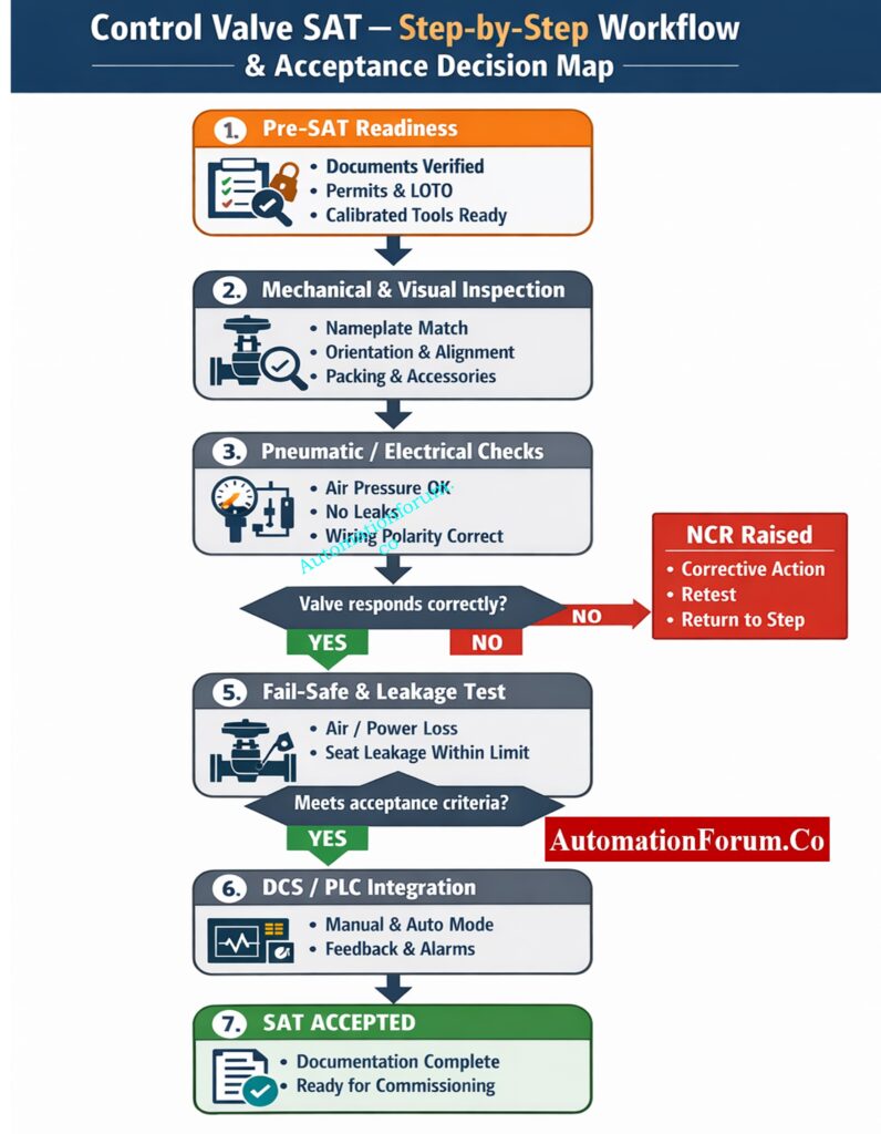
This SAT technique gives instrumentation engineers, commissioning teams, and EPC practitioners a useful, ready-to-use protocol for checking control valves after they are installed and before they are put into use. It expands every activity into explicit, ordered bullet steps so technicians can execute tests reliably, document results, and resolve failures efficiently. This version is written to be used directly on site clear, actionable, and focused on outcomes and safety.
A Control Valve Site Acceptance Test (SAT) is the final technical gate before a valve enters service. SAT confirms that what left the factory still performs correctly after transport, installation, and connection to air, power, and control systems. Problems caught at SAT are far cheaper and safer to fix than those found during commissioning or under process conditions. A rigorous SAT improves reliability, reduces startup delays, and protects safety instrument functions.
Purpose: Verify installation, mechanical integrity, actuator/positioner performance, signal and power wiring, fail-safe action, seat/passing leakage as required, and DCS/PLC integration prior to introducing process fluid.
Scope: This includes all control valves (globe, rotary, ball, butterfly), actuators (pneumatic, electric, hydraulic), positioners (pneumatic, electro-pneumatic, smart/HART), limit switches, solenoids, tubing, and any other I/O that is needed to control systems.
Pneumatic valves depend on correct air pressure and quality. Validate supply and tubing before functional tests.
Air source and FRL checks:
Measure pressure at the filter-regulator with a calibrated gauge; set to vendor recommended (commonly 4-6 bar / 60-90 psi).
Check that the FRL bowl is dry and drain it if you need to.
Tubing and connector checks:
Make sure the tubing is the right size and material, that there are no kinks, and that it has the right slope where condensation drains are supposed to go.
Leak detection on pneumatic side:
Pressurize actuator and positioner ports; apply soap solution to all fittings and joints; check for bubbles.
Air stability test:
Cycle the valve slowly while monitoring inlet pressure for significant drops (indicates undersized supply or leaks).
Check accessory operation:
Manually operate solenoid valves where possible to confirm switching and exhaust routing.
Fail-safe action must be precise and reliable for safety functions and emergency shutdowns.
Simulate air loss: With valve in service conditions simulated (or safe test condition), isolate instrument air and observe valve move to fail position.
Simulate power loss (electric actuators): Turn off the motor supply and make sure that any spring-return or mechanical override works as it should.
Verify solenoid actions: Turn off the solenoids and check that their exhaust or vent routing allows for safe movement.
Measure fail time: Keep track of how long it takes to get to the fail position and make sure it is within the permitted range for safety function timing.
Confirm final state: Check that the valve locks or stays in a safe state, as needed by safety philosophy (for example, stays closed unless manually reset).
Check to see if the valve seat and packing match the standards for isolation and leakage.
Test Isolation & Safety Precautions
Make sure that the upstream and downstream lines are physically separate and that the testing follow all safety and permit rules.
Step-by-Step Seat Leakage Test
Put the test pressure at the rated or agreed-upon level with the valve fully closed. Then, watch the pressure downstream and use a soap solution at the stem and bonnet to find the paths of leakage.
Inspect packing area under pressure for visible seepage. Slight seepage may be acceptable depending on packing type document and compare with project limits.
Acceptance Criteria & API Comparison
Compare observed leakage to contract or API class limits. If leakage is higher than allowed levels, find out what’s causing it (broken trim, wrong seating, foreign material) and fix it.
After fixing problems, do leakage tests again to make sure the fixes worked.
Make sure that all status and monitoring signals show the real state of the machine.
Position transmitter verification: At 0%, 50%, and 100% mechanical travel, check the 4-20 mA position feedback signal and make sure the scaling is right.
Limit switch checks: Check the limit switches by stroking the valve and turning on the limit switches to make sure the open/closed indicator and wiring to the DCS discrete input are correct.
Volume booster and relay function: If there is one, check that the volume booster works by sending quick stroke commands to make sure there is no lag or cavitation in the air supply.
Diagnostic logging: Record any fault codes or alarms presented by smart devices and resolve or escalate per procedures.
DCS/PLC Integration & Control Loop Interaction
Make sure that directives from the control room lead to correct valve behavior and feedback.
Manual Mode Verification From DCS
From the DCS, place valve in manual mode and send step changes; observe valve respond in the field and confirm feedback mirrors movement.
Auto Mode Dry Run & Loop Observations
Where safe, place loop in auto mode with simulated or constrained process variables; observe valve response to setpoint changes.
Tagging, Scaling & Alarm Verification
Confirm DCS displays correct tag, action, percentage open scale, and correct low/high calibration.
Loop behavior and stability
Look for undesired oscillation, hunting, or irregular response. If present, evaluate valve sizing, positioner tuning, or loop tuning.
Interlock & shutdown checks
Test cause-and-effect interactions where the valve participates in interlocks or safety trips (simulated where necessary).
Complete and accurate records turn field tests into acceptance that can be traced.
Record keeping: Keep track of test dates, people, instruments used (including calibration dates), and specific numeric measurements (pressures, timings, currents).
Non-conformance reports (NCR): Document any failures with root cause, corrective action, responsible party, and retest plan.
Device configuration records: Save positioner, transmitter, and smart device configurations and diagnostic logs.
Vendor/FAT certificates: Attach factory test certificates and calibration reports to the SAT dossier for the valve.
Acceptance statement: Prepare a clear handover statement describing test scope, results, outstanding issues, and commissioning readiness.
A thorough, planned SAT that follows the steps above gives commissioning teams the peace of mind that control valves will work as planned in the plant’s safety and control systems. A thorough SAT takes time, but it lowers the danger of expensive shutdowns, makes things safer, and speeds up the commissioning process. To make sure that commissioning and operations go smoothly, execute SATs with organized paperwork, calibrated equipment, and participation from people in different departments (instrumentation, operations, vendor).
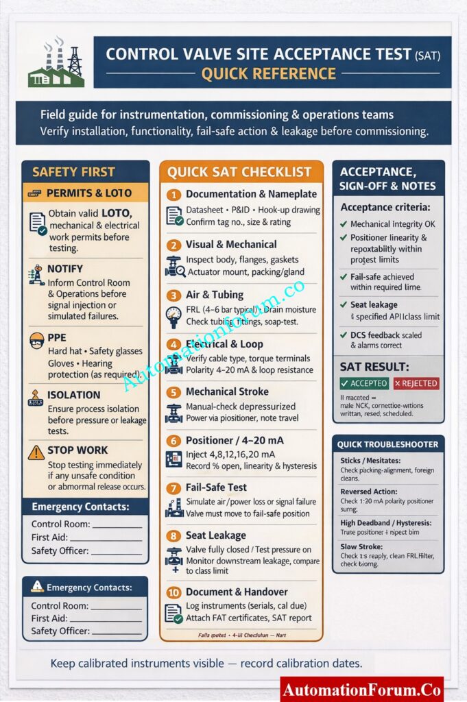
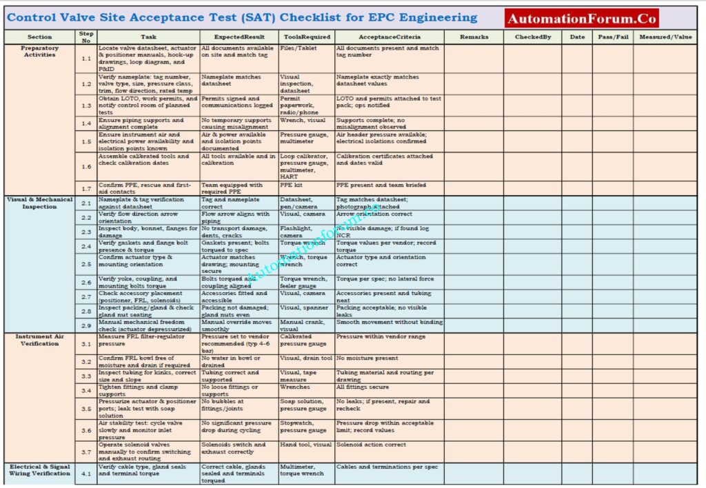
Control Valve Site Acceptance Test (SAT) Checklist
A Control Valve Site Acceptance Test (SAT) checklist is an organized, ready-to-use document that is used after installing the valve and before putting it into service.
This checklist enables the instrumentation and commissioning teams check the mechanical installation, actuator and positioner performance, air and electrical connections, fail-safe action, seat leakage, and DCS/PLC integration in a methodical way.
A complete SAT checklist cuts down on commissioning delays, makes things safer, and makes sure that control valves work exactly as they should.
Representatives from vendors and operations teams may also take part. All stakeholders sign off the SAT for commissioning readiness.
What is the full form of FAT and SAT?
FAT stands for Factory Acceptance Test. SAT stands for Site Acceptance Test. FAT is done at the manufacturer’s facility, while SAT is done at site.
What is SAT validation?
SAT validation is the documented confirmation that installed equipment meets design requirements. It proves that systems perform as intended under real site conditions. SAT validation is critical for quality assurance and regulatory compliance.
Typical range: 0.95-0.99 for flow meters | 0.85-0.95 for general applications
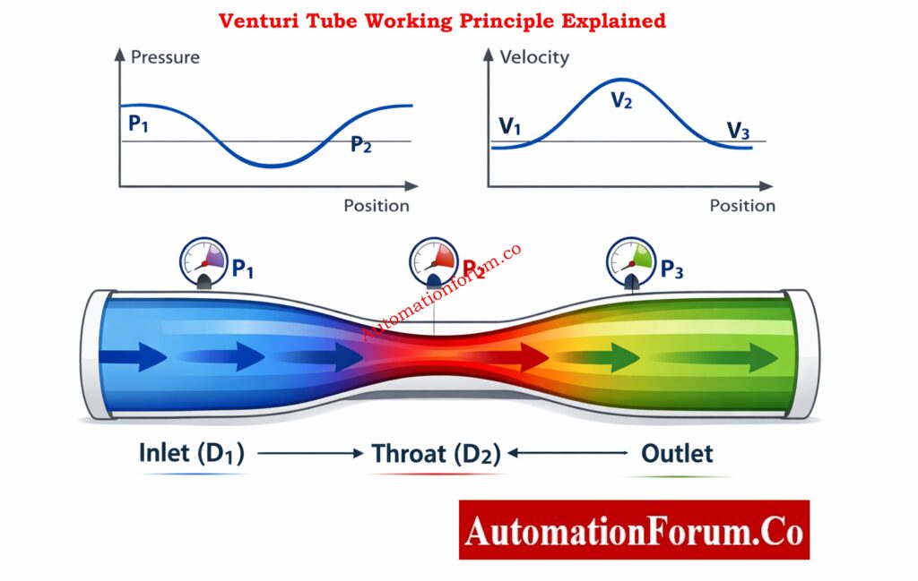
ℹ️ About Venturi Tube:
A precision flow measurement device that uses the Bernoulli principle. As fluid accelerates through the narrowed throat section, pressure decreases, creating a measurable pressure difference proportional to the flow rate. Ideal for clean, non-corrosive fluids.
📋 Applicable Standards:
• ISO 5167-4:2022 – Measurement of fluid flow by means of pressure differential devices – Part 4: Venturi tubes
• ASME MFC-3M-2004 – Measurement of Fluid Flow in Pipes Using Orifice, Nozzle, and Venturi
• BS EN ISO 5167-4 – Venturi tube flow measurement standard
• API MPMS Chapter 14.3 – Concentric, Square-Edged Orifice Meters & Venturi Meters
📋 Design Standards:
• ISO 5167-4:2022 – Venturi tubes for flow measurement
• ASME MFC-3M-2004 – Fluid flow measurement using Venturi meters
• BS EN ISO 5167-4 – British/European Venturi tube standard
• API MPMS 14.3 – Venturi meters for custody transfer
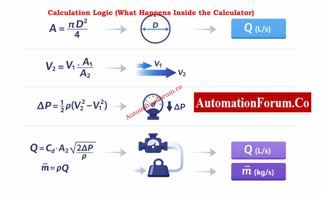
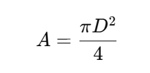
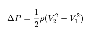
The Advanced Venturi Tube Flow Calculator is a computerized engineering tool that uses the well-known principles of continuity and Bernoulli’s equation to figure out the mass flow,pressure drop, velocity, and fluid flow rate. This calculator is more than just a number engine; it uses proven equations, unit conversions, visual representations, and graphs to help engineers understand how flow works inside a Venturi tube.
This guide goes over how to use the calculator in detail, what each input and output parameter represents, how the calculation logic works, and where this tool may be used in real life. The explanations follow worldwide standards and are designed for students, instrumentation engineers, automation professionals, and process designers.
Refer the below link for Instantly Convert DP to Flow – Try This Interactive Calculator
A Venturi tube is a device that measures flow by measuring differential pressure (DP). It has :
An inlet (upstream pipe)
A converging cone
A throat (minimum diameter)
A diverging cone (pressure recovery section)
When fluid flows into the throat, its speed goes up and its static pressure goes down. You can figure out the flow rate accurately by measuring this difference in pressure.
Best-Practice Usage Tips for Venturi Tube Flow Calculation
Always check that D₂ is less than D₁.
Use density levels that are reasonable for the conditions in which you are working.
Check to see if ΔP is within the limitations of the transmitter.
Use Cᵈ values that are based on standards for the final design.
The Advanced Venturi Tube Flow Calculator is a great tool for both learning and engineering that connects theory and practice. It helps engineers comprehend not just what the flow rate is, but also why it acts the way it does by combining verified equations, unambiguous inputs, detailed outputs, and visual analysis.
When used appropriately, this calculator may help you make better design choices, operate more safely, and learn more deeply, making it a useful tool for modern process and automation engineering.
Frequently Asked Questions on Venturi Tube Flow Calculation
How to calculate Venturi flow?
Using the continuity equation and Bernoulli’s principle, you can figure out how Venturi flow works. We measure the pressure drop between the inlet and throat to find the speed. Then, the flow rate is figured out by multiplying the throat area by the fluid speed.
How does a venturi tube measure flow?
By making the pipe’s throat smaller, a venturi tube monitors flow by speeding up the fluid and lowering the pressure. The flow rate is directly related to the difference in pressure between the intake and throat. Standard equations turn this difference in pressure into flow.
What is the formula for flow in a tube?
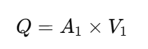
The basic flow formula for a tube is Q = A × V, where Q is the volumetric flow rate, A is the cross-sectional area, and V is the speed of the fluid. This equation is only true for steady, incompressible flow. It comes from the principle of continuity.
What is the volumetric flow rate of a venturi tube?
The volumetric flow rate of a venturi tube is the amount of fluid that flows through the pipe in a certain amount of time. You can figure it out by using the throat area, pressure differential, fluid density, and discharge coefficient. Most of the time, the outcome is given in m³/s or L/s.
How to calculate flow rate formula?
You may find the flow rate by calculating Q = A × V, where A is the area of the pipe’s cross-section and V is the average speed. In differential pressure devices such as venturi tubes, flow is generated by pressure drop rather than direct velocity. Both techniques are founded on the idea that mass stays the same.
What is the formula for Venturi suction?
The pressure differential at the neck caused by the higher speed is used to figure out Venturi suction. Bernoulli’s equation says that increased speed means lower static pressure, which is where the suction pressure comes from. This idea is employed in vacuum generators and ejectors.
Control valve hunting is a common and expensive problem in process control systems that lowers the quality, safety, and profitability of products. This advanced quiz focuses on real-world troubleshooting in a variety of fields, including oil and gas, chemicals, power, utilities, pharmaceuticals, and refineries. It helps engineers spot patterns that indicate problems, figure out what is causing them, and choose the best course of action. Some of the topics are tuning, stiction, sizing issues, I/P and air supply problems, positioner feedback, process dead time, and strategy flaws. Each question based on a scenario is like what happens in the field during commissioning, start-up, and operations. This helps teams improve their diagnostics, reduce oscillations, and speed up repairs, which makes the plant more reliable.
25 Advanced Scenario-Based MCQs on Control Valve Hunting Troubleshooting Scenarios
Emergency valves are safety-critical devices that decide whether a plant lives or dies in an incident. Properly designed and tested Emergency Shutdown Valves (ESDVs) and Emergency Blowdown Valves (EBDVs) protect people, the environment, and assets in oil & gas, petrochemical, refinery, and power facilities.
Despite similar names, ESDV vs EBDV are often misunderstood – and that misunderstanding can be fatal. This article explains the difference between isolation and depressurization, the fail close vs fail open philosophy, real-world testing practices, and the verification steps every instrumentation and safety engineer must enforce.
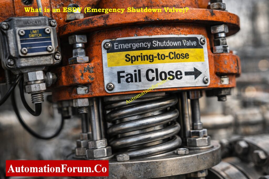
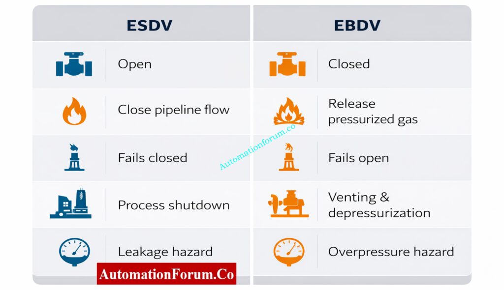
An Emergency Shutdown Valve (ESDV) isolates process flow to remove fuel or feedstock from a hazardous area; it is designed to fail closed (ESDV fail close).
ESDV Definition and Purpose
An ESDV is a safety critical valve whose primary role is to isolate process streams. It prevents hydrocarbons, steam, or other hazardous materials from feeding an accident. ESDVs are major elements of any ESD and fire & gas system.
Typical Applications of ESDV
Inlet isolation at unit boundaries (e.g., CDU feed)
Fuel supply shutdown to burners and heaters
Emergency isolation of transfer and loading lines
Isolation upstream of critical rotating equipment
Normal vs Emergency Operation of an ESDV
Normal condition: Valve is open to allow process flow.
Emergency condition: Valve must close immediately upon a trip signal (fire, gas detection, HI-HI pressure, loss of containment).
Why ESDV Is Designed to Fail Close
Fail-close mitigates escalation by cutting off the source of fuel or feed. If instrument air or power is lost, the actuator’s stored energy drives the valve to the closed position, minimizing inventory and stopping further hazard growth.
An Emergency Blowdown Valve (EBDV) vents pressurized fluids to a safe disposal path (usually flare) to rapidly depressurize equipment; it is designed to fail open (EBDV fail open).
EBDV Definition and Purpose
EBDVs are dedicated valves used to rapidly depressurize vessels, skids, and piping during an emergency. The goal is to remove stored energy and reduce the risk of rupture, BLEVE, or jet fire.
Typical Applications of EBDV
Blowdown of compressors, separators, and reactors
Emergency depressurization of storage tanks and pipe racks
Fast depressurization on detection of high temperature or fire on equipment
Normal vs Emergency Operation of an EBDV
Normal condition: Valve is closed and isolated from the flare/vent header.
Emergency condition: Valve opens to route mass to a flare or vent, reducing internal pressure and stored energy.
Why EBDV Is Designed to Fail Open
Fail-open ensures depressurization continues even if control power or instrument air is lost during the incident. The protected outcome is avoiding catastrophic mechanical failure and limiting overpressure-related harm.
A fail-safe design means the valve defaults to the safest state when components fail. “Safe” depends on the hazard:
Isolation hazards → safe = closed (ESDV).
Stored energy hazards → safe = open (EBDV).
Why ESDVs and EBDVs Have Opposite Fail Actions
ESDVs and EBDVs address different hazard vectors. ESDVs remove the ongoing source of energy; EBDVs remove energy already trapped inside equipment. This fundamental difference explains the opposite fail actions.
Fail Action Selection Based on HAZOP, LOPA and SIL
Correct fail actions should be outcomes of HAZOP, LOPA, and SIL studies. These instruments drive valve selection, actuator type, proof-test intervals, and the interlocking logic required by modern safety instrumented systems.
Valve Selection and Actuator Design Considerations
Actuator Selection for ESDV (Fail Close Valves)
ESDV: Use spring-to-close actuators (air-to-open / spring-to-close) and confirm spring energy exceeds worst-case process backpressure.
Actuator Selection for EBDV (Fail Open Valves)
EBDV: Use spring-to-open actuators (air-to-close / spring-to-open) sized for rapid opening under pressure.
Positioners, Limit Switches and Valve Status Indication
Fit local mechanical flags and independent position transmitters.
Use redundant limit switches for safety-critical status reporting.
Ensure HMI and valve tag detail the fail action clearly.
SIL Valves and Proof Testing Requirements
Include ESDV and EBDV in SIL assessments where applicable. Define proof-test frequency, diagnostic coverage, and functional test procedures in the Maintenance Plan.
Common ESDV and EBDV Design and Maintenance Mistakes
Typical Engineering and Commissioning Errors
Assumption over verification: Relying on vendor defaults instead of testing.
Wrong solenoid logic: Using de-energize-to-open when the design required de-energize-to-close.
Bypass left in place: Temporary bypass during commissioning left active – defeats safety function.
Incorrect actuator orientation: Spring installed in wrong orientation; actuator fails opposite way.
Poor documentation & training: Operators unaware how valve should behave in fail mode.
Real-World Consequences of Incorrect Fail Action
Mis-specified fail action has led to uncontrolled blowdowns, ruptured vessels, and fires. These are not valve faults alone they are system-level failures in design, procurement, and verification.
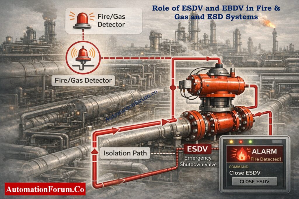
Role of ESDV and EBDV in Fire & Gas and ESD Systems
How ESDVs Respond to Fire and Gas Detection
In a properly designed plant, the Emergency Shutdown Valve is directly linked to the fire & gas system. Upon confirmed fire or gas detection, the ESD logic forces the ESDV to close immediately. This action isolates fuel sources feeding the incident area, limiting fire size and preventing escalation into adjacent units.
From a process safety perspective, ESDV fail close is non-negotiable in hydrocarbon service. If an ESDV fails open during a fire, the fire & gas system loses its primary mitigation function, regardless of how advanced the detection is.
The Emergency Blowdown Valve plays a complementary role. While ESDVs stop incoming energy, EBDVs remove trapped energy already inside equipment. During fire exposure, rapid depressurization via EBDV fail open reduces vessel wall stress and lowers the risk of catastrophic rupture.
Coordinated Action of ESDV and EBDV
This coordinated action isolation by ESDV and depressurization by EBDV is the backbone of modern process safety valves design.
Timing and Stroke Speed – A Critical Safety Parameter
Why Valve Stroke Time Matters
Fail action alone is not enough. Stroke time is a critical parameter:
ESDVs must close fast enough to cut off fuel before escalation.
EBDVs must open fast enough to depressurize before metal temperature weakens pressure boundaries.
Many incidents occur not because the valve failed to move, but because it moved too slowly. Stroke time requirements should always be validated during FAT and SAT.
Typical Industry Stroke Time Expectations
ESDV closure: often 5-10 seconds, depending on line size and hazard.
EBDV opening: often 2-5 seconds for critical equipment.
These values must align with HAZOP and SIL assumptions – not vendor convenience.
Refer the below link test your knowledge with SIS Quiz for Instrumentation & Safety Engineers
Human Factors and Safety Culture Impact on Emergency Valves
Common Human-Related Safety Risks
Even perfectly designed safety critical valves can fail the plant if human factors are ignored. Common human-related risks include:
Incomplete understanding of fail close vs fail open valve philosophy
Poor handover between project and operations teams
Lack of periodic functional testing awareness
Building a Strong Verification Culture
Plants with strong safety records treat valve fail action verification as a mandatory ritual – not a commissioning formality. Engineers, technicians, and operators must all know:
What the valve does
How it fails
Why it must fail that way
This shared understanding transforms ESDVs and EBDVs from hardware items into true process safety barriers.
ESDV isolates flow by closing; EBDV depressurizes by opening. They are part of the same safety family but act opposite to mitigate different hazards.
What is the difference between blowdown valve and shutdown valve?
A shutdown valve (ESDV/SDV) isolates process flow by closing during an emergency. A blowdown valve (BDV/EBDV) opens to depressurize equipment by venting to flare or vent. Shutdown stops incoming energy, while blowdown removes stored energy.
What is the difference between fail open and fail close valves?
A fail close valve closes automatically on loss of air, power, or signal to isolate the process. A fail open valve opens automatically on failure to release pressure or energy. Fail action is selected based on process safety requirements.
An SDV (Shutdown Valve) is a general shutdown valve used for operational or process trips. An ESDV (Emergency Shutdown Valve) is safety-critical and tied to the ESD or fire & gas system. All ESDVs are SDVs, but not all SDVs are ESDVs.
What is the difference between ESDV and SDV?
An ESDV is designed for emergency conditions and usually requires SIL-rated performance. An SDV may be used for normal shutdowns or process interlocks. ESDVs have stricter testing, fail action, and safety integrity requirements.
What is the difference between SDV and BDV?
An SDV isolates flow by closing the valve during shutdown. A BDV (Blowdown Valve) opens to depressurize vessels or piping during emergencies. SDVs isolate hazards, while BDVs reduce pressure and stored energy.
What is an ESD valve?
An ESD valve (Emergency Shutdown Valve) is a safety-critical valve that isolates hazardous fluids during emergencies. It is normally open and designed to fail close on loss of power or air. ESD valves are key components of ESD and fire & gas systems.
What is ESD 1 and ESD 2?
ESD 1 is a partial shutdown affecting specific equipment or process sections. ESD 2 is a full plant or unit shutdown during major emergencies like fire or explosion risk. The classification depends on plant safety philosophy and hazard severity.
Final Safety Reminder – ESDV vs EBDV Is a Safety Philosophy, Not a Checkbox
ESDV and EBDV are siblings in the safety architecture same family, same urgency, but opposite emergency intent. The single most important control you have as a designer, engineer, or technician is verification: design intent written on P&IDs and delivered through FAT/SAT, with documented proof that the valve will behave as intended under loss-of-power or loss-of-air conditions.
In process safety, clarity beats assumption. The ESDV vs EBDV decision is not a checkbox it’s a safety philosophy implemented through engineering, procurement, testing, and operations. Use rigorous FAT/SAT, confirm fail-close vs fail-open at installation, and lock proof testing into your maintenance regime.
Above all: train your teams, document every test, and never accept a “this is how the vendor supplied it” answer without witnessed verification. Safety-critical valves require system thinking not component thinking.
Getting the fail position wrong is not a valve issue it is a safety system failure.
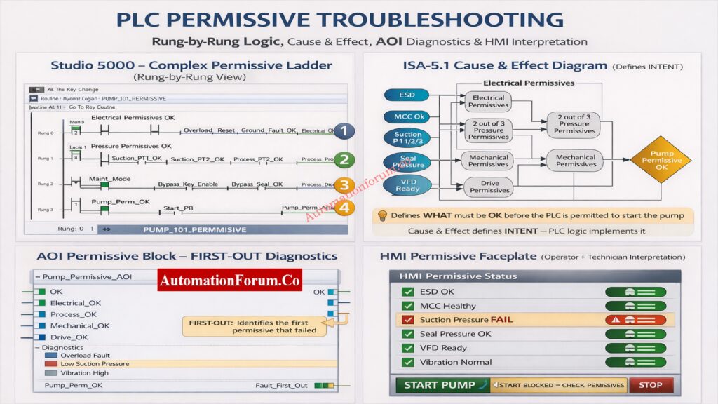
Why PLC Permissive Logic is Critical in Process Plants
In today’s process industries, like oil and gas, chemicals, power generation, water treatment, and pharmaceuticals, PLC permissive logic is the safety net that keeps people, equipment, and production goals safe. A pump, compressor, or fan may look like it’s ready to go, but the PLC won’t let it start unless all of the predefined permissive criteria are met.
Instrument engineers deal with permissive logic problems every day. A single broken pressure transmitter, an MCC feedback that isn’t lined up right, or an AOI that isn’t set up correctly can bring down a whole unit. This paper is meant to help engineers understand, fix, and explain PLC permissive logic in a systematic, real-world way using ladder logic, the Cause & Effect philosophy, AOI diagnostics, and HMI interpretation.
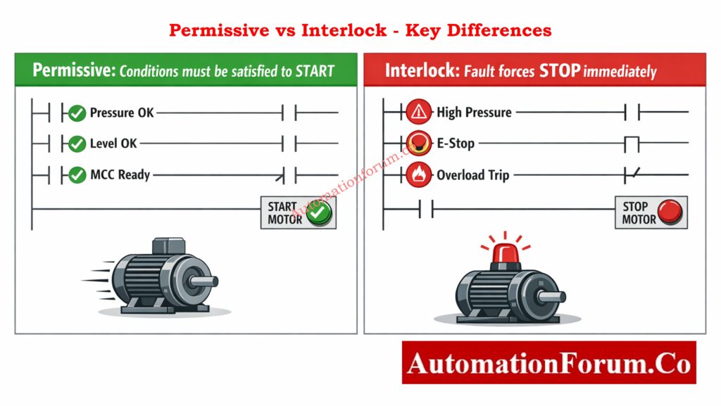
Before an action may happen, PLC permissive logic says that a series of logical conditions must be TRUE. Most of the time, the action is to start a pump, open a valve, or turn on a drive.
PLC permissive logic is a set of logical criteria that must all be TRUE before a PLC will let something happen, such starting a pump, turning on a motor, or opening a critical valve.
Permissives are purposely cautious. The PLC stops the start command if even one permissible condition fails. This design philosophy puts safety, protecting equipment, and keeping processes stable ahead of making things available right away.
Some common examples of permissive situations are:
When you’re trying to figure out what’s wrong with a machine, it’s important to know the difference between permissives and interlocks. Permissives tell you why a machine won’t start, while interlocks tell you why it stopped.
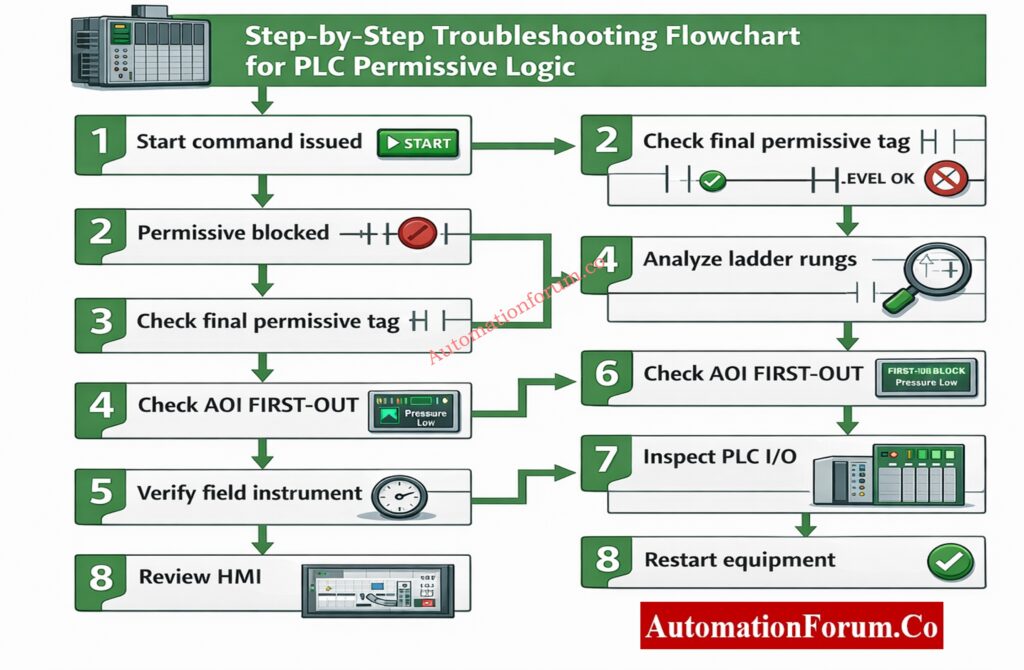
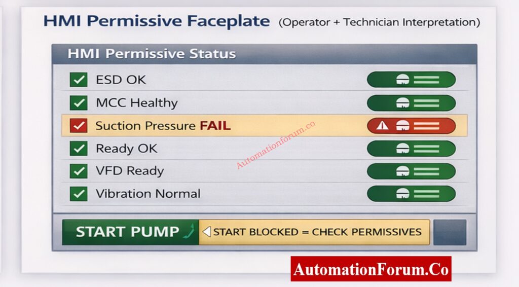
Step 1: Confirm the Start Is Blocked by Permissive Logic
Check if the inability to start is really because of permissives before opening PLC logic or checking instruments.
Some common signs are:
Operator issues a start command
No motor rotation or drive start
HMI message such as “Start Blocked – Check Permissives”
At this point, don’t make any assumptions. Make sure that permissive logic is to blame and that the problem is not caused by a power loss, a breaker trip, or a mechanical lock-out.
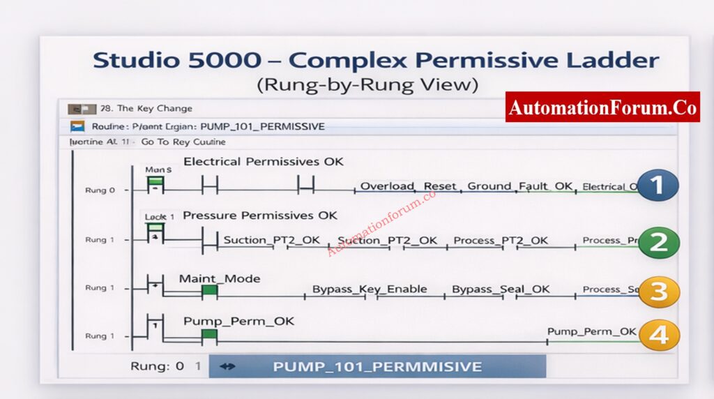
Step 3: Analyze the Permissive Ladder Logic Rung-by-Rung
A permissive ladder is usually set up with each rung being a logical series of conditions.
Permissive logic is normally divided into logical rungs, each representing a group of conditions. Analyze them sequentially.
Electrical Permissive Rung
This rung typically verifies:
MCC health or contactor feedback
Reset of the emergency stop circuit
Reset the overload relay
Ground fault fixed
If any signal is FALSE, check to see if the problem is real or if it is caused by wiring problems, broken auxiliary contacts, or PLC input module problems.
This rung evaluates process safety conditions such as:
Suction pressure within limits
Discharge pressure below high limit
Flow present
Many plants use 2-out-of-3 voting logic for critical pressures. Always evaluate the voting result, not just individual transmitter readings. A single failed transmitter may not block the start, but two failed transmitters will.
Always troubleshoot from left to right and top to bottom, exactly how the PLC scans logic. When a final output is false, trace each upstream rung to find the first rung where the logic evaluates to false.
Put the ladder into logic forcing mode and toggle the suspected inputs one by one (for example, force the suction pressure OK tag) and observe the effect on FIRST‑OUT. But remember: never force a tag without proper safety permissions and clear communication with operations.
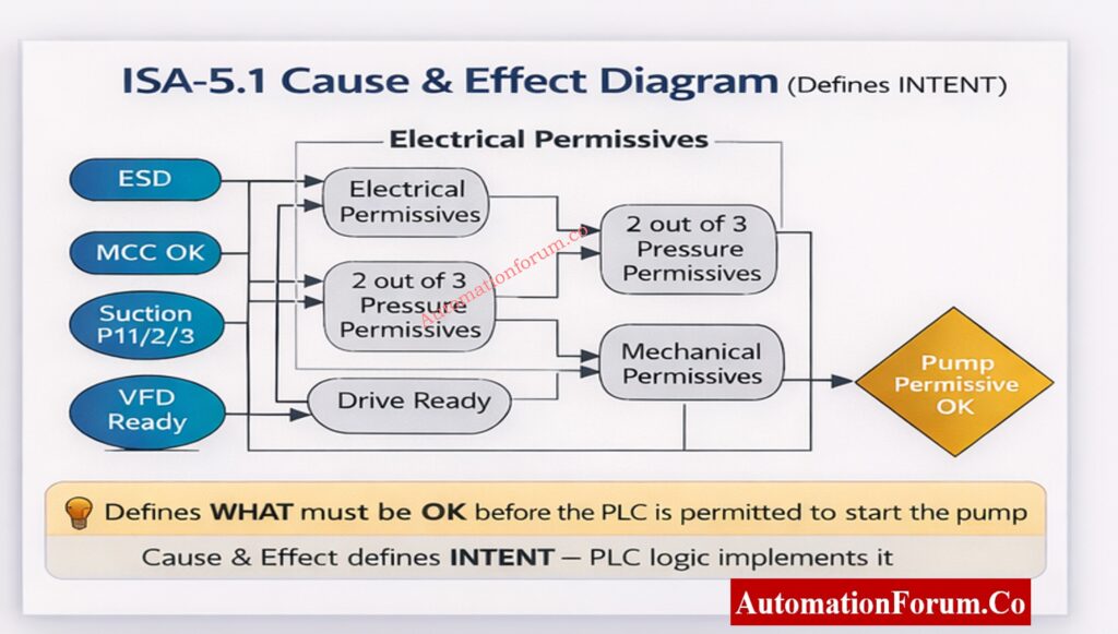
Step 4: Verify Design Intent Using Cause & Effect Diagram
The Cause & Effect (C&E) diagram, as per ISA-5.1, defines WHAT must be OK before the PLC is allowed to act. It does not describe code it describes intent.
Why Cause & Effect Important
Serves as the contractual logic reference between process engineers and control engineers
Links process safety to control logic and HMI behavior
Ensures consistency across PLC, DCS, and emergency systems
Cause & Effect (C&E) diagrams define what conditions must be satisfied before a start is permitted. They represent the safety and operational intent of the system.
Confirm that every permissive in the ladder exists in the C&E diagram
Check that the voting rationale satisfies the C&E definition.
Find any undocumented permissions that were added during changes.
If there is a difference between C&E and PLC logic, it should be seen as a big design problem. Always keep the C&E and ladder logic in sync. Use code comments or a mapping document that links each C&E bubble to a PLC tag and AOI parameter so field technicians can quickly find the implementation.
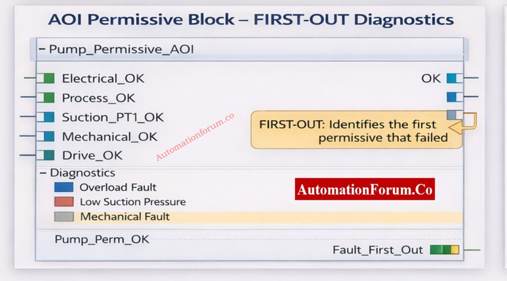
An Add-On Instruction (AOI) is a reusable logic block that standardizes permissive logic across equipment. AOIs can contain inputs, outputs, and internal tags which makes them ideal for consistent FIRST‑OUT behavior.
FIRST-OUT Logic Explained
FIRST-OUT logic captures the first permissive that fails, even if multiple permissives fail later. The AOI sets a Fault_First_Out tag and often a code or priority bitset that the HMI can interpret.
Easier operator guidance because HMI can show the likely cause
Better trending and reliability metrics because the first fault is logged
Implementation notes
Use timestamped fault registers in AOIs to capture when the first failure occurred.
Include a ‘clear’ or ‘acknowledge’ mechanism that does not erase historical logs- use a separate event log for permanent records.
Prioritise safety-related permissives (e.g., ESD) higher in FIRST‑OUT priority than operator convenience permissives.
Modern PLC systems use Add-On Instructions (AOIs) to standardize permissive logic. A well-designed AOI includes FIRST-OUT diagnostics, which record the first permissive that failed.
Read the FIRST-OUT diagnostic tag
Identify the first permissive that transitioned to FALSE
Troubleshooting Scenarios for PLC Permissive (Real-World Examples)
Below are common real-world scenarios with quick diagnosis steps and recommended fixes. Use these as a quick reference during field troubleshooting.
Scenario A – Suction Pressure Permissive Failure
Symptoms: HMI shows Pump_Perm_OK = FALSE and FIRST-OUT indicates Suction_Pressure_FAIL. Immediate checks: Read live suction pressure trend; inspect the impulse line and filter/strainer; check the transmitter healthy bit. Likely root causes & fixes:
Blocked suction strainer – clean or replace strainer.
Transmitter calibration drift – calibrate or replace transmitter.
Impulse line air trapped – bleed the impulse line. Verification: Restore signal, confirm reading on HMI, clear FIRST-OUT, reattempt start.
Scenario B – MCC Healthy Feedback FALSE
Symptoms: MCC_Healthy = FALSE even though motor starter appears energized. Immediate checks: Inspect motor starter auxiliary contact, check MCC bus voltages, and confirm breaker position. Likely root causes & fixes:
Auxiliary contact welded or stuck – replace or repair contactor.
Advanced Trending, Analytics and Preventive Maintenance Strategy
Use historian data and rudimentary analytics to turn events that are allowed into reliability improvements that you can act on. Make the following trends and dashboards:
First-Out Frequency Chart: This chart shows how many FIRST-OUT events happen per tag each month. It helps find people who do it more than once.
Time-to-Fix Trend: The time between the FIRST-OUT timestamp and the restoration. This shows MTTR for permissive issues.
Voting Logic Failures: Keep an eye on cases where voting outputs stopped a start. This can assist find problems with sensor dependability.
NOTE: Set up historian exports for the AOI FAULT_FIRST_OUT tag, the final permissive tag, and the critical transmitter health bits. Make a simple dashboard that lets you filter by equipment, shift, and root cause.
Business benefit: Trending shows long-term problems (such bad sensor installation, electrical noise, or repeated use of a bypass) that single incident reports don’t catch.
Advanced Trending, Analytics, and Preventive Maintenance Strategy
Calibration timetable for sensors: every 3 to 6 months for critical transmitters (suction/discharge pressure, flow), depending on how bad the process is.
I/O integrity checks: Every three months, verify the termination blocks, torques, and grounding.
Check your drive regularly: look over your event record once a month and check your cooling system once a quarter.
HMI and AOI audit: Once a year, check that the AOI diagnostics and HMI faceplates show the most up-to-date logic and C&E.
Keep track of PM work in the CMMS and link work orders to FIRST-OUT events that can check how well PM works.
Following ISA standards and local laws lowers the chance of legal problems and accidents.
Adding sophisticated trending, preventative maintenance, and a systematic RCA process to your permissive troubleshooting technique will make your plant stronger. This article’s steps help instrumentation engineers find and fix permissive-based start failures while keeping safety and compliance in mind.
These minor behaviors, like following the checklist, following safety rules, and writing down anything you notice, can help you work faster and give operators and engineers more confidence.
A PLC permissive is a logical condition that must be TRUE for a PLC to let something happen, such turning on a pump or motor. Before starting up, it makes sure that the electrical, process, and mechanical conditions are all safe.
How to troubleshoot PLC problems?
When you debug a PLC, you check the power, I/O status, logic conditions, and communication health. When there are problems with starting, engineers check permissive logic, FIRST-OUT diagnostics, and field instrument signals one at a time.
What does it mean to start permissive?
Start permissive means that all the necessary requirements are met, thus the PLC can accept a start instruction. If any permissive is FALSE, the PLC stops the equipment from starting up to keep it from becoming dangerous.
What is the difference between permissive and interlock?
A permissive lets something happen when it is safe, while an interlock stops or prevents something from happening when it is not safe. Permissives let things start, while interlocks keep things safe.
What are the three types of interlocks?
There are three main types of interlocks: electrical, mechanical, and process interlocks. They work together to keep people and equipment safe from dangerous working circumstances.
What does permissive signal mean?
A permitted signal is a confirmation signal that shows that a necessary condition has been met. The PLC lets the operation go ahead when all of the permissible signals are TRUE.
JB Grouping in Process Industry Instrumentation Systems
JB grouping is one of the most important yet frequently overlooked engineering tasks in projects involving industrial automation and instrumentation. If the project is in oil and gas, chemical plants, power generation, pharmaceuticals, cement, steel, or water treatment facilities, the quality of the installation, the speed of commissioning, the safety of the plant, and the efficiency of long-term maintenance all depend on how well the junction boxes are grouped.
JB grouping may sound very technical, but it’s really just about having wiring make sense, making maintenance easy, and making commissioning go well. If you don’t arrange your JB grouping well, it might cause signal noise, grounding problems, frequent loop check failures, extra effort on site, and longer startup delays. A well-designed JB grouping philosophy, on the other hand, makes sure that the wiring is clean, the signals are reliable, the troubleshooting is faster, and all project and safety criteria are met.
This article is a full, useful, and SEO-friendly reference to JB grouping. It covers what it is, why it’s important, how to design it, safety issues, signal separation, using 3D tools, best practices, frequent mistakes, and examples from real process plants.
What Is JB Grouping in Instrumentation Engineering?
Definition of Junction Box (JB) Grouping in Industrial Automation
JB grouping is the process of putting field instruments, actuators, analyzers, and electrical signals into the right junction boxes (JBs) based on engineering logic, safety categorization, signal type, and physical location.
JB grouping defines:
Which field instruments terminate in which junction box
How many signals are assigned to one JB
How signals are segregated inside the JB
How cables are routed from field instruments to control systems
The basic goal is to have structured wiring, short cables, less interference, quick troubleshooting, and safe functioning.
Why JB Grouping Is Critical in Industrial Automation Projects
Impact of JB Grouping on Instrument Installation and Cable Routing Efficiency
When you install, putting the JBs together correctly makes it easier to route cables and keeps trays from getting too full. When instruments from the same area or piece of equipment are logically grouped together, it is easier and faster to draw cables, and there is less danger of mis-termination.
Role of JB Grouping in Faster Commissioning and Loop Checking
JB grouping is very important for commissioning. Engineers can do the following using well-grouped JBs:
Find loops fast
Follow signals effortlessly
Find problems without having to open more than one JB.
Many commissioning delays happen not because the instruments are broken, but because the JB groups are set up wrong and the terminals are planned wrong.
Effect of JB Grouping on Signal Integrity and Control System Reliability
Noise can have a big effect on analog transmissions. Putting analog, digital, and power-related signals together in the wrong way can cause:
Signal fluctuation
Unstable readings
False alarms
Long-term signal stability and accurate process control depend on correct JB grouping.
JB Grouping Requirements for Safety, Hazardous Areas, and Code Compliance
JB grouping must precisely follow:
Hazardous area classification
Intrinsic safety requirements
Voltage separation rules
Not being able to organize JB correctly can cause safety violations, inspections to be turned down, and big operational concerns.
Key Design Criteria for JB Grouping in Instrumentation Engineering
Instrument Location and Area-Based Junction Box Grouping
Knowing where the instruments are physically is one of the first steps in JB grouping. It would be best if you put instruments that are in the same process unit, skid, or equipment area into junction boxes that are close to each other.
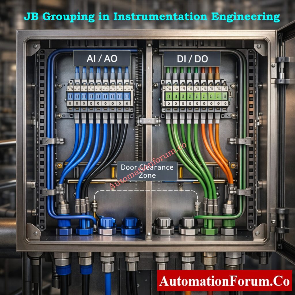
Separation of Analog and Digital Signals in Junction Box Grouping
Grouping of junction boxes to separate analog and digital signals
One of the most fundamental rules for JB grouping in instrumentation is to put analog and digital signals in separate junction boxes.
AI and AO are examples of analog signals. They are low-level signals that can be affected by electrical noise. Digital signals like DI and DO require switching operations that might cause interference.
Keeping analog and digital signals in different JBs:
Prevents signal interference
Improves control loop stability
Keeps wiring clean and organized
Simplifies troubleshooting
In a lot of EPC projects, DI and DO signals are also put in distinct JBs, based on the client’s and project’s standards. This may add more JBs, but it makes the system much clearer and more reliable.
Voltage Level Separation in JB Grouping (ELV, LV, and IS Circuits)
JB grouping must always take voltage levels into account. Some common voltage ranges are:
Extra Low Voltage (ELV)
Low Voltage (LV)
Intrinsically Safe (IS) circuits
If you don’t separate multiple voltage levels in the same JB, you could have insulation problems, noise problems, and safety problems.
Intrinsically Safe (IS) and Non-Intrinsically Safe (NIS) JB Grouping Philosophy
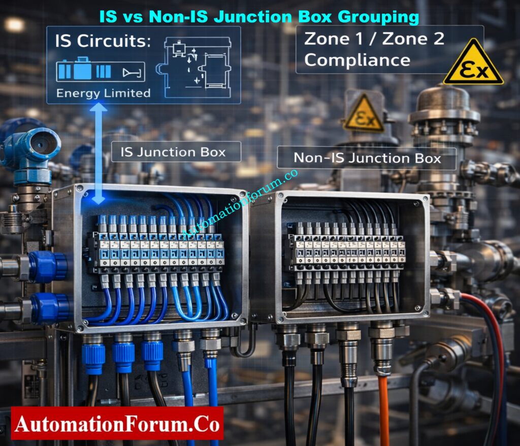
IS vs NIS Junction Box Grouping for Zone 1 and Zone 2 Areas
Even when there is a malfunction, Intrinsically Safe (IS) circuits are made so that energy is limited to keep things from catching fire. IS JBs are often used for:
Analog transmitters in dangerous places
Digital inputs from field switches in dangerous areas
Instruments linked via safety barriers or isolators
Non-Intrinsically Safe (NIS) is a safety idea that says circuits should be built so that they don’t make sparks or get too hot when they are working normally. NIS, on the other hand, doesn’t protect as well as IS, hence it should only be utilized if area classification and project requirements allow it.
Important Practical Rules for IS and Non-IS Signal Segregation
Both analog and digital transmissions must follow IS and NIS criteria.
For instance:
Even though it is merely a digital signal, a limit switch in a dangerous location must end in an IS-rated JB.
A typical mistake on sites is to mix IS and non-IS signals in the same JB without properly separating them. This often means that work has to be done again during commissioning.
It is best to use specific IS junction boxes that are clearly marked, have blue terminals, and are kept separate from non-IS wire.
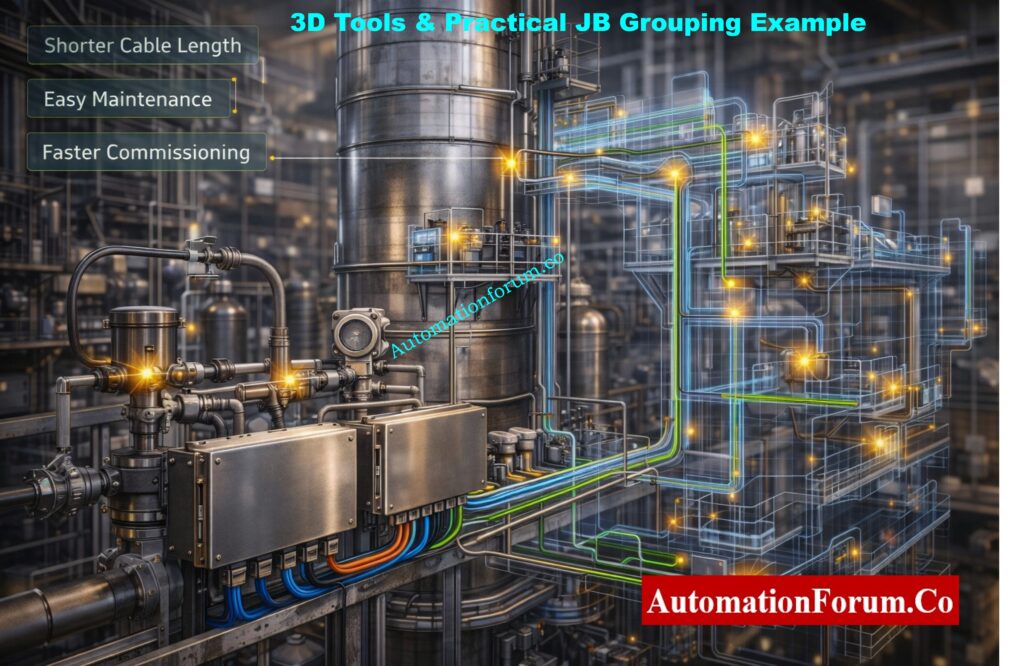
Role of 3D Engineering Tools in Junction Box Grouping Design
How 3D Tools Like Nevis Improve JB Grouping Accuracy
3D design tools like Nevis are becoming more and more important to modern instrumentation and automation engineering since they help with precision and synchronization throughout thorough engineering. 3D tools let engineers see the whole plant environment in a realistic and integrated way, which is different from typical 2D drawings.
Engineers can see well with 3D models:
Field instruments and their exact installation locations
Cable trays, ladders, and routing paths
Structural beams, platforms, and supports
Equipment layouts and access clearances
This level of visibility changes JB grouping from a theoretical documentation exercise to an actual engineering choice that is ready for the site. This cuts down on assumptions and design mistakes before construction starts.
Advantages of 3D-Based JB Grouping for EPC and Site Execution
Using 3D engineering tools has a number of practical benefits for successful JB grouping:
Put junction boxes near groups of field instruments to shorten cable length and cut down on voltage drop and signal loss.
Put instruments in groups depending on where they will actually be installed, not on the rough positions suggested on 2D drawings.
Make sure the cable tray routing is as efficient as possible to avoid tray congestion and too many cable crossings.
Cut down on the total length of the cables, which will save money on installation labor, trays, and cables.
Stay away from conflicts with pipes, equipment, and building parts so that you don’t have to do any extra work on site.
Make site installation less confusing by clearly defining JB locations and coordinating them with other disciplines.
Engineers can make better, faster, and more reliable judgments by using 3D tools like Nevis instead of trying to figure out where JB is from 2D drawings.
JB Grouping Checklist Before Finalizing Instrumentation Design
Before locking in the JB grouping design for an instrumentation project, the following checks must be carefully looked at to avoid having to do work again, safety problems, and delays in commissioning.
Engineering and Safety Checks for Junction Box Grouping
Check the area categorization to see if the installation site is a safe region or a dangerous area, like Zone 0, Zone 1, or Zone 2.
Make sure that all project specifications, client standards, and relevant international codes are followed. JB grouping rules may be different for each project.
Make sure that Intrinsically Safe (IS) and Non-Intrinsically Safe (non-IS) circuits are completely separate, both physically and at the terminals.
Check that the voltage levels are separate and that ELV, LV, and IS circuits are not all in the same junction box.
Signal Segregation and Cable Selection Checks in JB Grouping
Check that all signal types, including as AI, AO, DI, DO, RTD, and thermocouple signals, are properly separated to avoid interference and wiring problems.
Choose the right cable type for each signal, like a pair or triad arrangement, and make sure it has the right level of protection, such being insulated or armored, depending on the needs of the project.
Make sure each junction box has enough spare terminals so that you may be flexible when you first set it up and make changes in the future.
Make sure to include extra cable pairs so that you may add more instruments, expand the system, or change the loop without having to pull new cables.
Installation, Accessibility, and Maintenance Considerations
Make sure that junction boxes are easy to get to for installation and regular maintenance, and that they don’t need scaffolding or special access tools.
Make sure you choose the right gland based on the type of cable and the region classification to make sure it is protected from mechanical damage and the environment.
Make sure there is enough room for the internal wiring inside the JB so that it can bend properly, end neatly, and be safe to operate in.
Make sure that the terminal numbers and tags are clear and consistent, and that they match the loop diagrams and wiring designs.
Environmental, IP Rating, and Mechanical Requirements for JBs
Choose the right IP rating for the junction box based on the weather, chemicals, dust, or being outside.
Depending on how likely it is to corrode and the atmosphere of the factory, pick the right JB material, like stainless steel, GRP, or aluminum.
Make sure that the earthing and bonding are done correctly, with a connection between the gland plate, enclosure, and earth terminals.
Practical JB Grouping Example from a Chemical Process Plant
Distillation Column Instrumentation – JB Grouping Process Scenario
Think about a chemical process plant’s distillation column area, which has the following field instrumentation and devices:
For continuous pressure monitoring, pressure transmitters are put on column trays, overhead lines, and reboiler circuits.
Temperature transmitters, such as RTD and thermocouple sensors, that measure the temperatures of the process at different stages of the column
Control valves with positioners are used to control the flow of feed, reflux, and bottom product.
Level transmitters are put on the bases of columns and reflux drums to keep the level accurate.
Limit switches on valves and dampers for feedback on position and interlocks
Recommended JB Grouping Approach for Field Instruments
A useful and easy-to-implement JB grouping method for this area would be:
One specialized junction box for analog transmitters, installed near the distillation column to keep cable length short and make the signal more stable.
A separate junction box for digital signals from limit switches, which keeps them distinct from analog loops and makes it easier to find faults.
A separate Intrinsically Safe (IS) junction box for instruments that are put in dangerous places and meets all of the requirements for Zone 1 or Zone 2.
A separate junction box for thermocouple signals keeps electrical noise and interference from other types of signals away.
This method of grouping JB in a systematic way cuts down on the amount of cabling needed, makes the signal better, and makes loop inspection and commissioning a lot easier.
Common JB Grouping Mistakes Observed During Site Execution and Commissioning
People often make the following mistakes during site execution and commissioning, thus you should prevent them:
Putting both analog and digital signals in the same junction box might cause signal noise, readings that aren’t steady, and problems with troubleshooting.
Mixing IS and non-IS signals without properly separating them, which can lead to safety violations and being turned away during inspection
Not following the rules for digital signals in dangerous areas, thinking they don’t have to follow the laws for safety.
Not provide spare terminals or cable pairs, which will cause big problems when you need to add to or change things in the future.
Commissioning Engineer’s Pro Tip on Junction Box Grouping
From what I’ve seen in real life, many startup delays are due by wrong JB grouping instead of broken instruments. Before installation starts, always check JB grouping against loop diagrams and I/O lists. It’s much cheaper to fix problems during the design phase than after the fact.
Why Proper JB Grouping Is Essential for Safe and Reliable Industrial Automation
JB grouping in industrial automation and instrumentation is a lot more than just connecting wires. It is a very important engineering task that affects safety, dependability, commissioning time, and the cost of the plant during its whole life.
Engineers may make JB groups that are useful, safe, and ready for the future by following the rules for hazardous areas, using contemporary 3D tools like Nevis, and separating signals correctly. Instrumentation engineers that engage in EPC, site execution, commissioning, and plant maintenance need to be able to master JB grouping.
A JB (Junction Box) is an enclosure used in instrumentation to join and end wires from field instruments like transmitters, switches, and control valves before sending them to control panels.
What is a Type 4 junction box?
A Type 4 junction box is a strong box that keeps dust, rain, splashing water, and water from hoses out. It can be used indoors and outdoors in industrial settings.
What is a JB in electrical?
A JB (Junction Box) is a safe way to connect, branch, or end power lines in electrical systems. It also protects connections from damage caused by the environment and machines.
Programmable Logic Controllers (PLCs) don’t immediately grasp things like temperature, pressure, flow, or level in industrial automation systems. PLCs process raw digital counts that come from analog input modules instead. Before these raw data may be used for monitoring, control, alarms, and safety logic, they need to be correctly changed into engineering units.
This is where a PLC Raw Count Calculator becomes a must-have tool for engineers. Even while newer PLC systems include built-in scaling instructions, experienced automation professionals still use external raw count calculators to check, confirm, and fix problems with analog signal scaling.
This article goes into great detail on the differences between PLC internal scaling blocks and a PLC Raw Count Calculator. It then gives real-world examples of how to use these tools for pressure, flow, and temperature applications. Finally, it gives useful tips for commissioning, maintaining, and troubleshooting.
Using linear scaling math, a PLC Raw Count Calculator turns raw analog input values from a PLC into useful engineering units. It also lets you get from engineering values to raw counts in the opposite direction.
Analog input modules turn electrical signals like 4–20 mA or 0–10 V into digital form and then give you raw counts. These numbers are based on:
Engineers may check scaling on their own with a PLC Raw Count Calculator, which lowers the chance of making expensive mistakes during commissioning and operation.
The bottom part of the raw range is often used for diagnostics in S7-1200 analog modules. Engineers who don’t know how this works often get temperature indications wrong. This is a typical mistake that a raw count calculator can help you avoid. Calculate Thermowell U-Length Accurately (ASME Tool): Thermowell U-Length Calculator | ASME PTC 19.3 TW-2016 Tool
Analog Fault Simulation Using a PLC Raw Count Calculator
Fault modeling is a big plus for a PLC Raw Count Calculator.
Common Simulated Conditions
3.6 mA → Under-range (broken wire, broken sensor)
21 mA → Out of range (short circuit, transmitter problem)
Why Fault Simulation Matters
Engineers can check the following via failure simulation:
Why Every Automation Engineer Should Use a PLC Raw Count Calculator
PLC internal scaling blocks accomplish important math, but they don’t make independent verification unnecessary. A PLC Raw Count Calculator gives you more information, trust, and validation across platforms than just using internal PLC logic.
This instrument is very important for the whole life cycle of an automated system, from design and commissioning to operation and maintenance. It is used for measuring pressure and flow, controlling temperature, and finding faults.
It is essential for any engineer who works with analog signals to know how to interpret and validate raw count scaling.
When an analog input module changes signals like 4–20 mA or 0–10 V into a digital value, that value is called the raw count in PLC. It shows the electrical signal in numbers before it is scaled. Later, raw counts are changed into technical
What are the 4 main parts of PLC?
The four basic pieces of a PLC are the power supply, the CPU (processor), the input modules, and the output modules. The power supply gives the PLC power, the CPU runs logic, the inputs read signals from the field, and the outputs control things like motors and valves.
How to calculate 4-20 mA scaling?
Linear scaling is used to figure out 4–20 mA scaling: Engineering Value = (Raw − RawMin) × (EngMax − EngMin) ÷ (RawMax − RawMin) + EngMin. This changes PLC raw counts into useful process quantities like °C, bar, or %.
How to check PLC inputs and outputs?
You can inspect PLC inputs and outputs by checking the I/O status online, forcing signals if you can, and checking the wiring in the field. During commissioning and troubleshooting, input LEDs, output LEDs, multimeter readings, and PLC diagnostics assist make sure everything is working right.
What are the 4 steps of PLC?
There are four steps in how PLC works: Input Scan, Program Execution, Output Update, and Housekeeping. The PLC receives inputs, runs logic, updates outputs, and does internal diagnostics all the while in a scan cycle.
What are 5 output devices?
Motor starters, solenoid valves, control valves, indicator lamps, and relays are five popular PLC output devices. These devices get signals from PLC output modules to control electrical and mechanical processes in industrial automation systems.
Why Gas Turbine Startup Interlocks and Trips are Critical
Starting up a gas turbine is the most dangerous part of the operation since the speed, temperature, and fuel energy release change quickly. To keep these hazards in check, turbine control systems use start permissives, interlocks, and safety trip logic that is always on. Before fuel is added, start permissives make sure that important auxiliary systems are ready. Trip logic safeguards the turbine from dangerous operating circumstances during acceleration and operation. If lubrication, fuel handling, speed feedback, or combustion monitoring don’t work right, it could cause serious mechanical damage or safety problems. So, for safe commissioning, dependable startup, and long-term turbine integrity, it is very important to fully grasp starter interlocks and trip test methods.
Gas Turbine Start Permissive, Interlock & Trip Test MCQs for Engineers


 Procedure - Step-by-Step Field Guide 1")