Why HART Diagnostics are Essential in Process Automation

In the world of process automation, measurement reliability is everything. When a pressure, level, or temperature reading drifts or fails, it doesn’t just disrupt production it can compromise safety, product quality, and plant uptime.

That’s why modern HART-enabled field instruments have become more than transmitters of process variables they’re intelligent sensors with built-in self-diagnostics that reveal the real health of your measurement loop.

Whether it’s a Rosemount 3051S, a HART temperature transmitter, or a smart flow meter, today’s devices continuously analyze their internal electronics, process conditions, and communication loops to tell you much more than a simple process variable.

Why HART Diagnostics Very Important

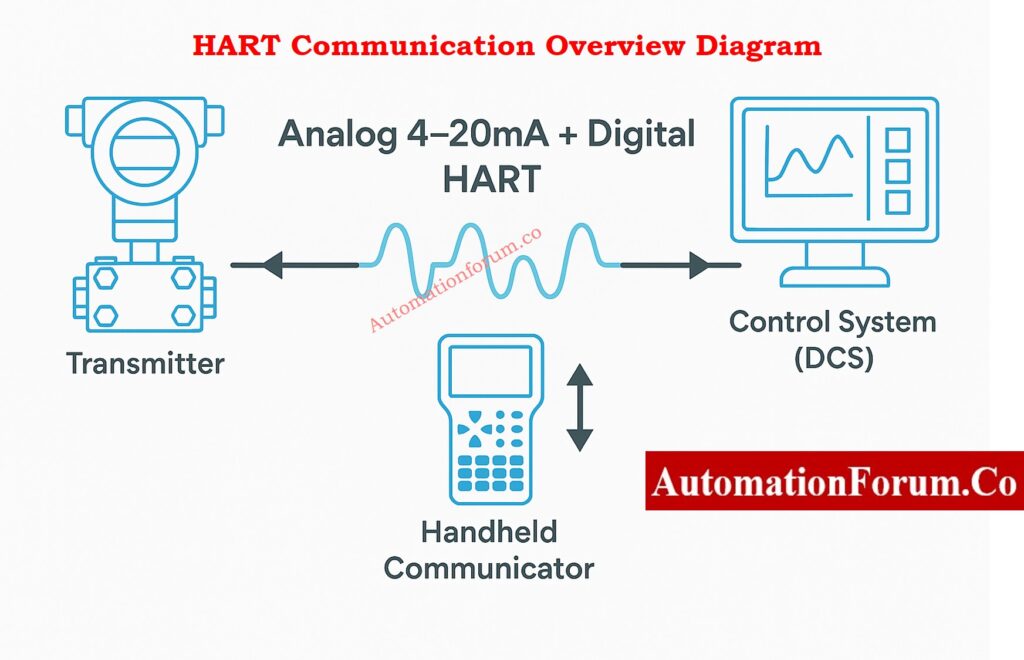
The Highway Addressable Remote Transducer (HART) protocol has existed since the 1980s. Initially, it was just a digital signal superimposed on the 4–20 mA loop to configure transmitters and read variables. But over the years, HART evolved into a powerful predictive maintenance tool.

Through its status bytes and command responses, a HART instrument can communicate:

• Whether its process variable is trustworthy,
• Whether it needs maintenance,
• And even whether a loop wiring or grounding fault exists.

When integrated into a DCS or asset management system (AMS), HART diagnostics help maintenance teams move from reactive to predictive maintenance anticipating failures before they affect production.
Get a complete overview from: What is HART Protocol?

Key Insights from HART Device Diagnostics

Modern HART devices generate a wealth of information beyond process values. Here’s what engineers can learn instantly:

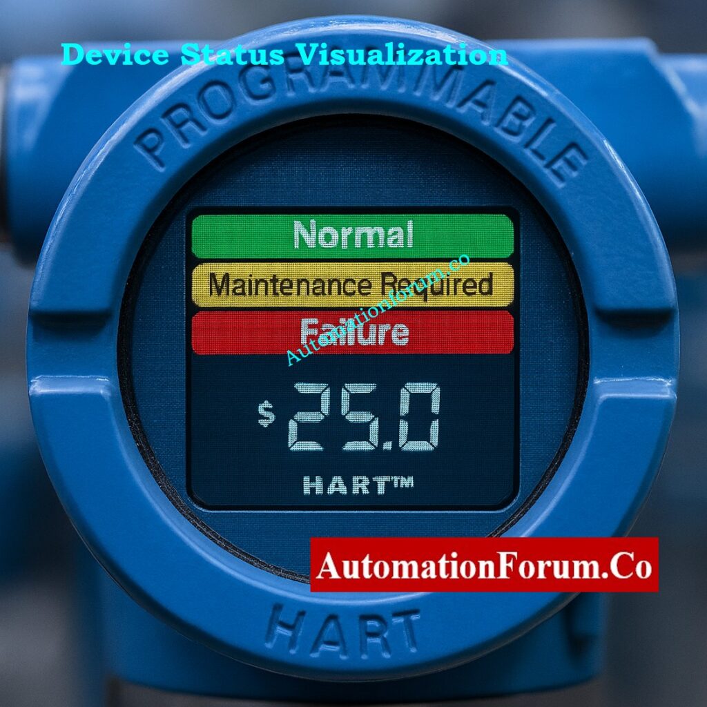
Device Status – Normal, Maintenance Required, or Failed

Each HART response includes a device status byte that tells whether the instrument is:

• Operating normally
• Needs maintenance
• Or has failed

This immediate visibility helps determine whether you can trust the process variable or if action is required.

Electronics Condition – Power, Grounding, and Temperature Checks

Continuous monitoring is done on internal factors such signal integrity, power supply voltage, and temperature. These tests can find problems with electronics, power, or grounding long before the instrument stops working.

Operational History – Tracking Service Hours and Calibration

Many transmitters keep track of the number of service hours, the last time they were calibrated, and the number of times they were turned on. This information helps in planning maintenance and proof-testing schedules in safety loops.

Sensor Integrity – Detecting Plugged or Damaged Sensors

Advanced devices detect plugged impulse lines, diaphragm wear, sensor drift, or process medium buildup. This ensures process readings reflect reality rather than mechanical or environmental problems.

Communication Health – Identifying Noise and Loop Issues

HART keeps an eye on the loop current, reaction time, and quality of digital communication all the time. The diagnostic data can show if there is noise, loose connections, or unreliable power.

Together, these insights form the backbone of a condition-based maintenance program that reduces unplanned downtime.
View the complete setup diagram in: Wiring Diagram for Pressure Transmitter Calibration in Workbench using HART

Power Advisory Diagnostics – Monitoring Loop Integrity

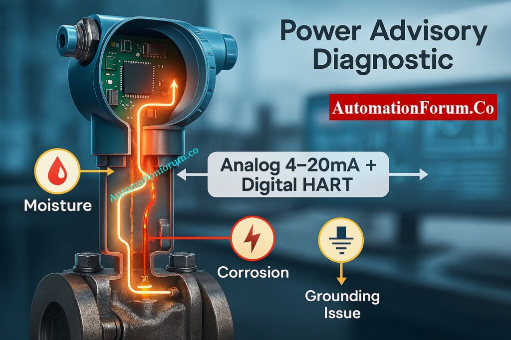
Electrical loop problems like corrosion, moisture ingress, or poor grounding are among the most common causes of transmitter failure.

The Rosemount 3051S Power Advisory Diagnostic uses real-time voltage monitoring to detect:

• Corroded terminals
• Water in terminal compartments
• Grounding or shielding issues
• Unstable power supplies

Instead of waiting for erratic readings, the transmitter issues detailed alerts with recommended actions. The result?
A maintenance technician can fix a corroded connection in a matter of minutes, which keeps the process from being interrupted for days.

Statistical Process Monitoring (SPM) – Seeing Beyond the Process Variable

What Statistical Process Monitoring Does

Statistical Process Monitoring (SPM): Looking Beyond the Process Variable

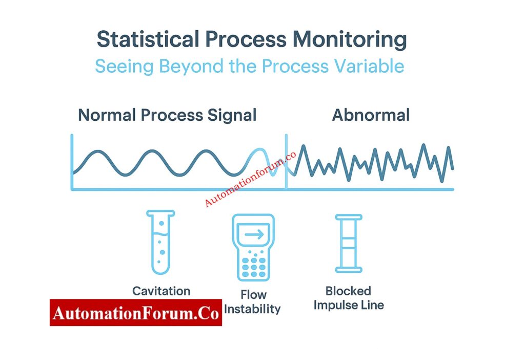
Standard alarms can only identify aberrant process conditions that Statistical Process Monitoring (SPM) can find by looking at noise patterns in the signal.

Common Issues Detected by SPM

SPM finds a lot of difficulties, such as:

• Flashing or cavitation in control valves
• Flooding of columns in distillation systems
• Blocked impulse lines or leaks in the process
• Loss of agitation in reactors
• Air or flame instability that becomes trapped

How SPM Turns a Transmitter into a Process Analyzer

SPM can tell operators about hidden problems like vibration, turbulence, or phase changes by comparing real-time signal patterns to baseline data.

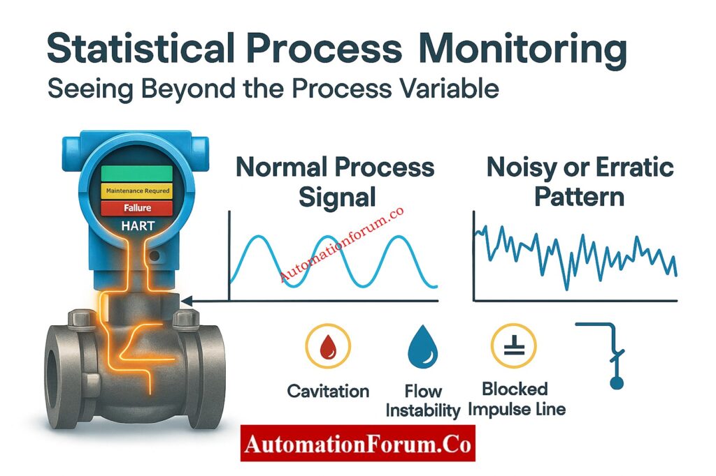
This changes a simple transmitter into a process analyzer that helps engineers find ways to make things run more smoothly and keep quality high.

Perform accurate calibration using: HART transmitter calibration procedure – For pressure transmitter

Safety-Certified Diagnostics – Reducing Proof Test Frequency

In Safety Instrumented Systems (SIS), each transmitter must be checked on a regular basis to make sure it works as IEC 61511 says it should.

Transmitters equipped with safety-certified diagnostics, like the Rosemount 3051S, increase diagnostic coverage by continuously verifying their sensing elements, electronics, and communication loops.

This greater Safe Failure Fraction (SFF) lets:

• Longer proof-test intervals
• Reduced maintenance workload
• Lower lifecycle cost

Operators can keep SIL compliance while cutting down on downtime when a transmitter can find problems on its own, like pressure spikes, loss of echo, or electrical drift.
Challenge your expertise through: Advanced HART Protocol Quiz: 25 MCQs with Detailed Explanations

Understanding HART Status Information

Every HART message includes two status bytes that form the foundation of its diagnostic capability.

Response Code (Byte 1) – Communication Integrity

Indicates whether communication was successful.

• 0x00 means “OK.”
• Other codes indicate to problems with processing commands or sending messages.

Device Status (Byte 2) – Operational Health

Reflects the operational condition of the field device.
It shows whether the transmitter is functioning correctly, in warning, or in failure.

Earlier HART versions treated these codes differently, but HART 7 standardized them so that every transmitter reports status consistently.

For example, a device status value of 0x90 (0x80 + 0x10) means the process variable is unreliable due to a process problem like a loss of echo.

Extended Device Status with NAMUR NE107 Codes

To simplify maintenance interpretation, modern transmitters use NAMUR NE107 condensed status codes.

This universal coding means that whether you’re using a pressure, level, or temperature transmitter, the DCS will interpret diagnostic messages consistently.

Device Variable Status – Can You Trust the Reading?

Each process variable in a HART device (like PV, SV, TV, or QV) has its own Device Variable Status.

• Good: Reading is valid.
• Bad: Fault or failure in measurement chain.
• Uncertain: Variable not guaranteed may be under test or simulation.

In short, before acting on a value, the control system can automatically decide whether that reading is trustworthy. This feature improves control loop integrity and prevents the use of corrupted process data.

Device Family Status – Process-Specific Fault Indicators

Different types of transmitters pressure, flow, level, or temperature use specific Device Family Status bits. These map diagnostics to process-specific meanings. For instance:

• A “loss of echo” in radar level devices,
• “Plugged impulse line” in differential pressure transmitters,
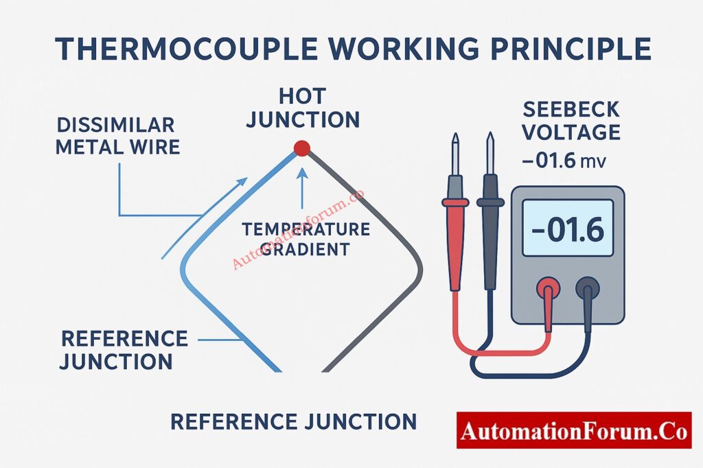
• Or “open thermocouple” in temperature devices.

HART Command 48 gets 25 more bytes of diagnostic data for deeper troubleshooting, with each bit linked to a distinct internal problem code. These correspond to the same messages displayed on the transmitter’s LCD screen.

With this level of detail, specialists can figure out if the problem is with the sensor hardware, the process interface, or the electronics.
Follow the best configuration methods in: Best Practices for Configuring HART Parameters in DCS Software

How HART Commands Carry Diagnostic Data

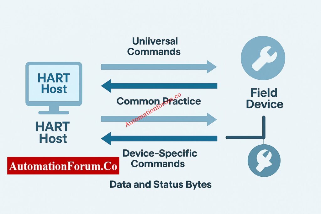
The HART protocol operates on a query–response model. The host delivers a command, and the device sends back data and information about its status.

There are three types of HART commands:

1. Universal Commands (0–30, 38, 48):
   All HART devices support this, which lets you read PVs, device info, and extended status.
2. Common Practice Commands (32–121):
   These are used by all device families for trimming, damping, or resetting.
3. Device-Specific Commands (128–253):
   These are set by the makers for their own diagnostic purposes.

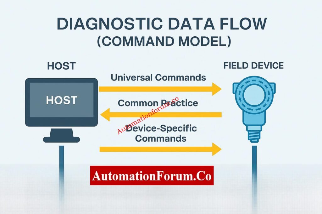
All responses include the two status bytes described earlier, meaning every command is both a data exchange and a health report.

Understand signal conditioning in: Why is a 250-Ohm Resistor Important for HART Communication?

From Hidden Data to Visible Intelligence

For decades, HART diagnostics remained hidden inside the device, accessible only through handheld communicators. Now, smart I/O cards and AMS software display this information directly in the control system.

This visibility answers crucial questions instantly:

• Can I trust the process variable?
• Is the transmitter in good health?
• Is this a problem with the process or the electricity?

Plants may make better decisions faster by using this diagnostic intelligence. This cuts down on troubleshooting time and increases uptime.

Refer the below link to Learn the fundamentals Explained: The Four Main Process Variables (PV, SV, TV, QV) in HART Transmitters – Complete Guide for Instrument Engineers

Integration with Asset Management Systems (AMS)

When you connect HART diagnostics to Emerson AMS Device Manager, Yokogawa PRM, or Honeywell FDM, they are immediately recorded, tracked, and trended.

This makes it possible:

• Dashboards for the health of all devices in one place
• Automatic notifications when things start to go wrong
• Maintenance documents that are ready for an audit

Engineers get alerts that they can act on, like “sensor drift increasing” or “loop voltage fluctuation detected,” instead of having to wait for an instrument to fail.

Real-World Example – Predictive Maintenance in Action

Imaging a differential pressure transmitter on a column for distillation. The impulse line starts to get clogged over time.

The HART transmitter sees a pattern of pressure changes that isn’t usual and sends out a “plugged line” signal.
Before any control deviation or trip occurs, maintenance isolates and cleans the line preventing an unplanned shutdown.

That’s predictive maintenance in action, enabled by HART diagnostics.

How HART Diagnostics Improve Safety, Productivity, and Cost

Improved Reliability

Self-checking all the time makes sure that only valid data gets into your control loops.

Predictive Maintenance and Early Fault Detection

Early detection of problems such sensor drift, unstable power, or process blockage.

Reduced Downtime

Finding faults faster cuts down on the time it takes to fix them and get back to normal.

Enhanced Safety and SIL Compliance

Better Safety Diagnostics that are safety-certified lower the number of proof tests needed while still meeting safety standards.

Lower Total Cost of Ownership

HART diagnostics pay for themselves many times over by extending maintenance intervals and stopping unexpected breakdowns.

Learning Objectives – What You’ll Gain from HART Diagnostics

By learning HART diagnostics, you will be able to: 

• Understand how status bytes send health information and how HART commands work.
• Understand NE107 alerts, response codes, and device status.
• Use SPM and Power Advisory to find problems with processes or loops early on.
• Combine diagnostics with DCS/AMS systems so you can watch them in real time.
• Make the safety system more reliable and cut down on the amount of work that needs to be done to keep it up.
  Master field installation using: Step-by-Step Guide for Installing and Commissioning HART and WirelessHART Devices for Engineers and Technicians

Turning Data into Diagnostic Intelligence

HART diagnostics turn your field equipment from silent data sources into smart protectors of process health.

Transmitters like the Rosemount 3051S make it possible to have a predictive, data-driven maintenance culture by checking the integrity of loops, monitoring statistical processes, and having safety-certified self-diagnostics.You get more than just numbers when you decode the rich diagnostic data that HART gives you. You can trust every loop, feel sure about every measurement, and make clear decisions about maintenance.

Test your troubleshooting knowledge with: Closed-Loop Control Valve Troubleshooting: HART, Fieldbus and Diagnostics Skills Quiz

FAQ on HART Transmitter Diagnostics

1. What are the benefits of HART communication?

HART communication mixes analog 4–20 mA signals with digital data. This lets you set up devices, troubleshoot them, and calibrate them from a distance. It improves accuracy, cuts down on maintenance time, and works with current wiring, making upgrades simple and cheap.

2. What is the main function of HART?

The basic purpose of HART is to provide two-way digital communication over typical 4-20 mA loops. This lets users get process, configuration, and diagnostic data from smart field equipment without stopping work.

3. Which of the following is a benefit of using the HART protocol?

One of the best things about using the HART protocol is that it lets you access instrument data and health diagnostics from a distance without having to run extra wires. This combines the durability of analog signals with the intelligence of digital signals to make plants run more efficiently.

4. What is the application of HART?

In process industries, HART is used to set up, keep an eye on, and fix problems with transmitters and smart instruments. It works with software used in oil and gas, power, chemicals, and water treatment industries.

Why Understanding Fieldbus and HART Matters in Industrial Automation

Communication between field instruments and control systems is very important in modern process automation. Over the years, HART (Highway Addressable Remote Transducer) and FOUNDATION Fieldbus (FF) have become two of the most prominent digital communication protocols in the instrumentation world.

Both platforms let you talk to field devices in an intelligent way, but their structures, data handling methods, and control capabilities are very different. For instrumentation and control engineers, especially those managing industrial networks in refineries, chemical plants, or power stations, understanding these differences is essential for effective design, commissioning, and maintenance.

Overview of HART Communication Protocol

What is HART (Highway Addressable Remote Transducer)?

The HART protocol came out in the early 1980s and is still one of the most popular standards for industrial communication. It adds digital communication to the standard 4–20 mA analog signal, which lets devices send both analog and digital data at the same time.

There are more than 10 million HART devices in use globally, making it the backbone of many legacy and brownfield plants.

How Does the HART Communication Protocol Work?

• HART superimposes a 1,200 bps digital signal (using FSK modulation) on the 4–20 mA analog loop.
• The analog signal still shows the main process variable (PV), and the digital layer conveys data about configuration, diagnostics, and subsidiary variables.
• HART works in a master/slave paradigm, which usually means that there is one main master (DCS/PLC) and one secondary master (handheld communicator or asset management software).

Learn about the four key process variables (PV, SV, TV, QV) in HART transmitters: Explained: The Four Main Process Variables (PV, SV, TV, QV) in HART Transmitters – Complete Guide for Instrument Engineers

HART Network Topology Explained

Most HART systems are point-to-point, which means that each device has its own pair of cables. HART also has a multidrop mode, which lets up to 15 devices share a single loop. However, only 3–4 devices are utilized in practice because the speed is too slow.

Key Advantages of HART Protocol in Process Industries

• Works with current 4–20 mA systems
• Technology that is easy to understand
• Handheld communicators are easy to set up and fix.
• Great for small updates in brownfield projects
• All major DCS/PLC vendors support it.

Explore the complete installation and commissioning guide for HART and WirelessHART devices: Step-by-Step Guide for Installing and Commissioning HART and WirelessHART Devices for Engineers and Technicians

Overview of FOUNDATION Fieldbus Communication Protocol

What is FOUNDATION Fieldbus in Process Automation?

FOUNDATION Fieldbus (FF) is a fully digital, two-way communication protocol that was first used in the late 1990s. It was made just for process automation. Fieldbus does away with the need for analog signals altogether. All data transfer, control, and diagnostics happen digitally over a single cable pair.

There are more than 10,000 systems in the globe that use Fieldbus devices.

How FOUNDATION Fieldbus Works – Architecture and Data Flow

Fieldbus has a real multidrop architecture, which means that more than one device can use the same wire segment. It sends power and digital signals over the same pair of wires, and each segment can accommodate up to 32 devices.

Fieldbus is over 25 times quicker than HART since it can send data at 31.25 kbps. This greater bandwidth makes it possible to control things in real time and talk to each other at the same time.

Key Features and Benefits of FOUNDATION Fieldbus

• Digital connectivity and the ability to control things in the field (CIF)
• Support for several variables and devices on one pair
• Time synchronization and event time-stamping at the device level
• Advanced diagnostics and predictive maintenance
• Vendor independence and interoperability
• Updates to firmware and settings online

HART vs FOUNDATION Fieldbus: Detailed Technical Comparison

Communication Architecture and Topology

Interpretation for engineers:
Engineers should know that HART is great for gradually updating old analog systems, while Fieldbus is better for new digital control designs where many instruments share a single network.

Understand why the 250-ohm resistor is critical in HART communication loops: Why is a 250-Ohm Resistor Important for HART Communication?

Power Supply and Energy Availability

HART devices can use about 35 mW of power, which is enough for basic diagnostics and sending parameters.

Fieldbus, on the other hand, can handle up to 2 A at 12–32 V, which gives modern processors and multivariable sensors a lot more power, even when they are in intrinsically safe (IS) mode.

With this increased power budget, the gadget can do more complicated things like statistical monitoring or valve signature analysis.

Data Communication Speed and Performance

• HART: The modest baud rate causes delays when polling hundreds of instruments because each one has to be asked one at a time.
• Fieldbus is a deterministic, planned communication structure (based on the publisher-subscriber paradigm) that makes sure updates happen quickly and in sync among devices.

Fieldbus lets network engineers use buses better and regulate loops in real time out in the field, which makes them less dependent on DCS scan rates.

Diagnostics, Predictive Maintenance, and Asset Monitoring

HART can diagnose problems with devices, including whether a transmitter has to be calibrated or has an internal issue.

Fieldbus, on the other hand, lets devices talk to each other, which makes it possible to monitor the health of the whole plant, diagnose valve problems, and do predictive analytics.

Advanced diagnostics running at 20–100 Hz in Fieldbus devices can detect subtle process or equipment issues that HART’s slower polling might miss.

Example:
A HART transmitter might report an intermittent fault that disappears before the system polls it. A Fieldbus device would push a timestamped event instantly to the host, ensuring no diagnostic data is lost.
Discover the essential Foundation Fieldbus installation and wiring best practices: Foundation Fieldbus Installation and Best Practices – Complete Guide for EPC and Maintenance Engineers

Control Strategies – Centralized vs Distributed (Control-in-the-Field)

This is a major differentiator.

• HART: Acts as a data layer; all control happens in the DCS using 4–20 mA loops.
• Fieldbus: Supports PID, logic, and arithmetic function blocks directly within field devices.

Control in the field reduces latency, improves reliability, and allows distributed control architectures  a key design advantage for future-ready plants.

Device Configuration and Plug-and-Play Flexibility

HART configuration typically requires a handheld communicator or DCS with HART-enabled I/O modules.
Fieldbus, on the other hand, supports automatic device recognition, online configuration, and firmware upgrades directly through the network.

Engineers can replace or upgrade a device without rewiring or recalibrating the loop  dramatically cutting commissioning time.

Multivariable Transmission Capabilities

While HART supports multiple variables (in digital mode only), Fieldbus devices can natively transmit several process parameters (e.g., flow, temperature, pressure) simultaneously and in real-time.

For instance, a single FF transmitter can potentially report level, density, and temperature on the same line, reducing the number of instruments and signal conditioners required.
Challenge yourself with this advanced Foundation Fieldbus communication quiz: Test your Knowledge on Foundation Fieldbus Communication Protocol: Advanced Quiz for Instrumentation Engineers

Commissioning and Maintenance Efficiency

Commissioning a HART-based loop requires physical verification, manual signal sourcing, and time-consuming calibration — typically up to 4 hours per loop.
Fieldbus commissioning, when engineered per FF AG-181 guidelines, can be up to six times faster because multiple devices are configured over the same segment, often in minutes.

This digital commissioning also integrates directly into asset management systems, simplifying documentation and maintenance scheduling.

Integration with Safety Instrumented Systems (SIS)

Currently, HART remains the practical choice for Safety Instrumented Systems, as FF-SIS adoption is still limited.
The Fieldbus Foundation has set standards for FF-SIF (Safety Instrumented Function) integration, which makes it possible for fully digital safety loops.

Firmware Upgrade and Future-Proofing Capabilities

• HART: Because of ASIC-based design, firmware upgrades need the electronics module to be replaced in person.
• Fieldbus: You can download firmware over the bus from a distance, which means you can add new features in the future without changing the hardware.
  

This feature makes Fieldbus a great long-term investment for plants that are going through a digital transition.
Understand the FISCO model for intrinsically safe Foundation Fieldbus H1 and Profibus PA systems: Fieldbus Intrinsically Safe Concept (FISCO) Model for Foundation Fieldbus H1 and Profibus PA

Practical Guidelines – When to Use HART and When to Choose Fieldbus

HART for Brownfield Projects (Existing Plants)

HART for Brownfield Projects (Plants that are Already There)

For incremental upgrading of old process facilities, HART communication is still the best and most affordable option. It works perfectly with the old 4–20 mA analog infrastructure, so factories may get the benefits of digital data without having to replace their existing wiring, junction boxes, or I/O cards.

HART helps maintenance teams enhance dependability and cut down on manual calibration work by supporting SIS (Safety Instrumented System) upgrades, device diagnostics, and remote configuration. Most plant technicians already know how to use HART portable communicators, so there is no need for a lot of retraining or software changes.

In brief, HART provides a low-risk modernization path that delivers enhanced insights while keeping proven analog reliability. 

Recommended for:

• Upgrading and retrofitting instruments and systems
• Changes to brownfields and small-scale plant expansions
• Updating SIS and combining device diagnostics
• Facilities that already have 4–20 mA infrastructure

 FOUNDATION Fieldbus for Greenfield Projects (New Plants)

For new installations and automation methods that put digital first, FOUNDATION Fieldbus is a good investment for the long term. As a totally digital, two-way communication protocol, it cuts down on the need for wire, control cabinet space, and marshalling hardware by a lot. This can save up to 40% on installation expenses.

Fieldbus lets you operate things in the field, so smart transmitters and positioners can run control loops locally. This reduces the strain on the DCS and speeds up the system’s reaction. It also allows condition-based maintenance and has built-in predictive diagnostics. This cuts down on unplanned downtime and maintenance expenses.

From design to commissioning, Fieldbus simplifies loop documentation, device calibration, and troubleshooting. It is ideal for plants that want integrated digital communication across the entire control hierarchy—forming the foundation for smart plants, Industry 4.0, and IIoT (Industrial Internet of Things) architectures.

Recommended for:

• Greenfield process units and new control systems
• Digital transformation and smart plant projects
• Facilities targeting reduced lifecycle cost and improved uptime
• Complex automation networks with advanced diagnostics and control.

Check out the detailed HART pressure transmitter calibration wiring diagram: Wiring Diagram for Pressure Transmitter Calibration in Workbench using HART

Key Advantages Summary – HART vs Fieldbus Side-by-Side

Follow this step-by-step guide on how to calibrate Foundation Fieldbus transmitters: How to calibrate Fieldbus transmitters?

Implementation Challenges with FOUNDATION Fieldbus

While Fieldbus offers impressive benefits, it’s technically complex. Engineers require training in digital network design, power conditioning, and function block configuration.
Initial setup issues, software bugs, and interoperability mismatches can occur if engineering practices or device testing are inadequate.

However, as device interoperability standards and engineering tools (like EDDL and FDI) have matured, FF adoption has become significantly easier and more reliable in recent years.
Get a clear explanation of the HART communication protocol basics: What is HART Protocol?

Comparison Table – HART Communication vs FOUNDATION Fieldbus

Prepare with our top 25 advanced Foundation Fieldbus MCQs for instrumentation pros: Foundation Fieldbus Network Protocol: Top 25 Advanced MCQ

The Role of Asset Management Integration in Digital Communication

For maximum benefit, both HART and Fieldbus should integrate into a Plant Asset Management (PAM) system.

HART in Plant Asset Management Systems

• HART is best for keeping track of basic calibration data and the status of devices.

FOUNDATION Fieldbus in Advanced Asset Analytics

• Fieldbus lets you keep an eye on conditions all the time, do predictive maintenance analytics, and back up your configurations automatically.

Integration Through OPC and DCS Platforms

Using OPC servers or native DCS interfaces to connect different systems makes sure that maintenance and reliability teams have access to real-time field intelligence.
Learn the fundamentals of Foundation Fieldbus H1 technology and communication layers: Foundation Fieldbus H1 Technology

Coexistence of HART and Fieldbus in the Future of Process Automation

For specialists who work in process automation, both HART and FOUNDATION Fieldbus is very important for industrial networking:

• HART remains the workhorse for legacy systems and incremental upgrades.
• Fieldbus is the basis for the next generation of digital plants. It provides real-time, coordinated, and power-efficient control from the field level up.

Digital technology is definitely the future of process automation. HART will be around for a long time, but Fieldbus technology has the scalability, diagnostic depth, and control flexibility that smart, connected, and efficient industrial operations need.
Start with the essential Foundation Fieldbus protocol basics explained clearly: Foundation Fieldbus Protocol Basics

FAQ on Fieldbus and HART Communication Protocols

What is the difference between Fieldbus and HART?

HART sends an analog 4–20 mA signal with a digital overlay for limited data. Fieldbus, on the other hand, is a fully digital network that lets devices talk to and control each other.

What is the difference between Fieldbus and Modbus protocol?

Fieldbus is a digital control network that works in real time and lets computers talk to each other. Modbus is a simplified master-slave protocol that is mostly used to send data.

What is the difference between Fieldbus and PROFIBUS?

Fieldbus has a lot of different types, and PROFIBUS is one of them. Fieldbus is the name for a group of industrial digital networks that includes PROFIBUS, Foundation Fieldbus, and others.

What is the difference between Fieldbus and Ethernet?

Fieldbus is made for deterministic, real-time control in automating processes. Ethernet is a universal data network that has been changed for use in industry with variants like PROFINET and EtherNet/IP.

Test your skills with this a Closed-Loop Control Valve Troubleshooting: HART, Fieldbus and Diagnostics

Refer the below link to Test your skills with this a Closed-Loop Control Valve Troubleshooting: HART, Fieldbus and Diagnostics Skills with our Quiz