- What Is Failure Rate (λ) in Reliability Engineering?
- Failure Rate in Predictive Maintenance and Asset Performance
- Failure Rate (λ) Calculator
- Failure Rate Formula and MTBF Calculator Explained
- Why Failure Rate Calculation Important in Industrial Maintenance
- How to use the Failure Rate Calculator (Step-by-Step Guide)
- Worked Examples of Failure Rate in Process Plants
- Applications of Failure Rate in Reliability and Maintenance Planning
- Who Should Use the Failure Rate Calculator?
- Common Mistakes in Failure Rate and MTBF Calculations
- Quick Application Map
- Failure Rate vs MTBF vs MTTF – Key Differences
- Related Reliability Calculators for Process Instrumentation
- FAQs on Failure Rate, MTBF, and Reliability in Process Industry
- Turning λ into Actions
- Example: From λ to Spare Parts
What Is Failure Rate (λ) in Reliability Engineering?
Definition of Failure Rate in Instrumentation Systems
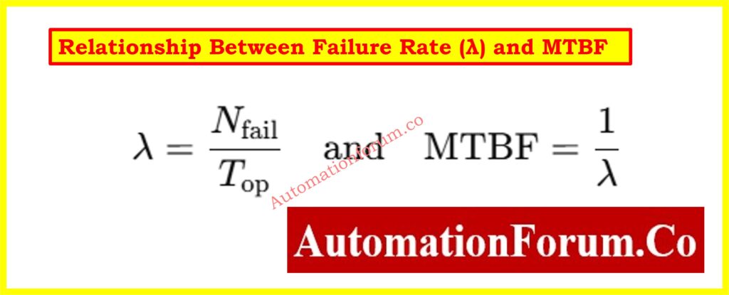
Failure rate (λ) indicates how often a repairable part or system is expected to fail per unit time while it is operating. It’s the instantaneous likelihood of failure during the “useful life” period and is the mathematical inverse of MTBF.
Failure Rate Formula
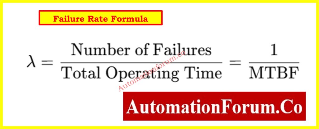
Units of Failure Rate (Failures/Hour, Failures/Year)
Units: failures/hour (commonly), failures/day, or failures/year be consistent.
Interpretation: A lower λ means better reliability; a higher λ means the item fails more frequently.
Failure Rate in Predictive Maintenance and Asset Performance
During normal operation (the “useful life” region of the bathtub curve), many electronic and instrumentation components can be modeled with a constant failure rate. In this region, reliability math uses an exponential distribution, where λ is constant and MTBF = 1/λ. That’s why λ is perfect for comparing the reliability of transmitters, control valves, analyzers, and PLC modules that run continuously in harsh process environments.
Failure Rate (λ) Calculator
The Failure Rate (λ) Calculator helps reliability, maintenance, and instrumentation engineers quantify equipment reliability using simple inputs: total operating time and number of failures. By converting these into λ and MTBF, you can predict downtime risks, optimize spare parts strategy, and support SIL/RCM studies.
Failure Rate Formula and MTBF Calculator Explained
Relationship Between Failure Rate (λ) and MTBF
Inputs
- Total Operating Time (hours): The cumulative time the asset was actually in service.
- Number of Failures: Count only true functional failures that required corrective maintenance.
Output
- Failure Rate λ (failures/hour)
- Equivalent MTBF (hours)
Calculation
Tip: If you already know MTBF, you can find λ right away by dividing 1 by MTBF.
Why Failure Rate Calculation Important in Industrial Maintenance
- Estimate the risk of downtime: Gives a number that shows how likely it is that an instrument will fail during a planned window.
- Benchmark vendors/equipment: A common way to measure how reliable different makes and models are.
- Optimize spares: Convert λ to expected demand for spare parts over a period.
- Support SIL/SIS analysis: λ is used in safety loop calculations for PFD_avg and availability.
- Perform maintenance first: Items with a high λ should be looked at, redesigned, or made less harmful to the environment sooner.
In 24/7 operations with heat, vibration, moisture, corrosion, or dirty utilities, even small differences in λ translate into many avoided trips and hours of saved downtime.
How to use the Failure Rate Calculator (Step-by-Step Guide)
Collect data
- From CMMS, historian, or shift logs, total the actual operating hours over the analysis period.
- Only count functional failures that can be fixed (don’t count planned shutdowns, upstream trips, or operator errors).
Inputs Required: Operating Time and Number of Failures
- Enter the total amount of time the machine has been running (in hours).
- Enter the number of failures.
Outputs: Failure Rate (λ) and MTBF
- The calculator gives you λ (failures per hour) and the same MTBF.
Interpret
- Lower λ is more reliable asset.
- Higher λ is investigate environment, duty cycle, or design; adjust PMs and spares.
Worked Examples of Failure Rate in Process Plants
Example 1: Control Valve Actuator in FCCU Air Line
- Operating Time: 16,000 hours
- Failures: 4 actuator diaphragm repairs
Compute λ:
λ= 4/16,000 = 0.00025 failures/hour
Equivalent MTBF :
MTBF= 1/0.00025 = 4,000 hours
Interpretation:
A failure rate of 2.5×10⁻⁴ failures/hour indicates one failure about every 4,000 hours. Use this to schedule inspections just before 4,000 hours, stock diaphragms/repair kits, and check whether ambient temperature, pulsation, or dirty instrument air are elevating λ versus the datasheet expectation.
Example 2: Steam Drum Pressure Transmitter
- Operating Time: 9,500 hours
- Failures: 1 (because of wet-steam impingement and contamination of the diaphragm)
To find λ, use the formula:
Λ = 1/9,500 = 1.0526×10⁻⁴ failures/hour
Equivalent MTBF:
MTBF = 9,500 hours
Interpretation:
Interpretation: A low λ means that the system is likely to be reliable on its own. Because the failure was caused by the process, think about using remote seals, snubbers, or better impulse line design to drop λ even more
Applications of Failure Rate in Reliability and Maintenance Planning
- Rank assets by λ to focus attention where it matters in Reliability-Centered Maintenance (RCM).
- Calculations for SIS and SIL: λ values (detected and undetected dangers) are used to calculate PFD_avg, proof test intervals, and SIF availability.
- Asset Performance Management (APM): Use Trend λ to make judgments about redesigning or replacing things.
- Planning for spare parts: Change λ into the number of projected failures each quarter or year to figure out how much stock to keep.
- Setting Up Baselines: Right after setup, set the initial settings for tracking KPIs.
- Contracts for maintenance or service level agreements (SLAs) commonly say what the maximum λ (or minimum MTBF) is.
Who Should Use the Failure Rate Calculator?
- Tune PM intervals and decide whether to do chores based on condition or time.
- I&C Engineers: Look at how different makes, models, and installations do in the field.
- Reliability Engineers: Measure how much better things are after improvements to the design or the environment.
- Plant and operations managers should plan for downtime and back up replacements with hard numbers.
- SIS Engineers: Use λD, or dangerous failure rates, in safety calculations.
- OEMs and service providers should measure the performance of their installed base against benchmarks.
Common Mistakes in Failure Rate and MTBF Calculations
- When mixing calendars with run-time, use the actual hours of operation, not the hours of downtime or shutdown.
- When counting failures, don’t include operator mistakes, upstream trips, or planned repair.
- Sets of data that are short: Very short intervals make λ noisy; for stability, average over longer spans.
- Ignoring causes: Track failure modes—process-induced issues inflate λ but have different remedies.
- Wrong metric:
- Use λ / MTBF for repairable items.
- Use MTTF for non-repairable items (e.g., fuses, certain sensors).
- Assuming constant λ blindly: The constant-λ (exponential) model holds mainly in the useful-life region, not in early infant-mortality or end-of-life wear-out phases.
Quick Application Map
| Equipment | Why λ Helps |
| Control Valve | Quantify actuator/positioner wear; set inspection and rebuild cadence. |
| Pressure Transmitter | Track drift/failures; plan calibration or seal replacement. |
| Solenoid Valve | Assess cycling fatigue; choose coil class and duty rating. |
| PLC Input/Output Card | Monitor electronic wear in high-density racks and hot enclosures. |
| Guided Wave Radar | Separate electronics vs. process-induced issues (coating, condensation). |
Failure Rate vs MTBF vs MTTF – Key Differences
| Metric | What it Means | Typical Use | Unit |
| λ (Failure Rate) | Frequency of failures per unit time | RCM, APM, SIL | failures/hour |
| MTBF | Average time between repairable failures | Availability & planning | hours |
| MTTF | Average time to failure for non-repairables | One-shot components | hours |
Conversions:
- Λ = 1/MTBF (for repairable items in useful-life region)
- MTBF and λ do not describe severity pair them with failure mode/impact data.
Related Reliability Calculators for Process Instrumentation
Helps engineers measure how quickly instrumentation faults are detected, supporting early-warning systems and predictive maintenance.
Best suited for non-repairable components such as fuses, sensors, and certain electronic devices, giving average time before failure.
Calculates the average time needed to restore a failed instrument, guiding spare part strategy and workforce planning.
Determines the average operating time between repairable failures, essential for preventive maintenance scheduling and SIL studies.
FAQs on Failure Rate, MTBF, and Reliability in Process Industry
Is a higher or lower failure rate better?
Lower λ is better. It means fewer failures per operating hour, resulting in less downtime and lower cost. A higher λ signals frequent failures and should trigger root-cause analysis, improved protection, or equipment changes.
What units should I use?
Use failures/hour for continuous processes. For reporting, you can scale to failures/10⁶ hours (FITs) or failures/year—just keep units consistent.
How do I compare two devices fairly?
Normalize both to the same units and ensure you used actual operating hours and the same failure definition. A/B test in similar environments where possible.
Can λ change over time?
Yes. Infant mortality (early life) and wear-out (late life) violate the constant-λ assumption. Trend λ over quarters/years to see shifts caused by environment, duty cycle, supplier changes, or PM strategies.
Turning λ into Actions
- High λ from process conditions: Add snubbers, remote seals, filtration, or heat tracing; relocate electronics; shield from vibration or EMI.
- High λ from component choice: Upgrade materials, IP rating, ingress protection, coil duty, or choose SIL-rated options.
- Stable, low λ: Safely lengthen PM intervals and lower stock levels.
Example: From λ to Spare Parts
If a factory has 12 identical solenoid valves that fail at a rate of 1.5×10⁻⁴ failures per hour,
Failures that are likely to happen each year:
12×λ×8,760=12×0.00015×8,760=15.8
Plan for 16 failures a year across the population and stock coils and kits accordingly.
 in process instrumentation. Improve reliability, optimize spares, and support SIL/RCM with real-world examples.)